Figure 2 - Draft 2
02_05_19
Note the YAML contains specifications for a github document and html. The best way to deal with this is to knit them separately from the knit menu. Otherwise the html has blurry plots and tends to delete the md cached plots unless you tell it to cache everything!
library(tidyverse)
library(cowplot)
library(broom)
library(modelr)
library(viridis)
library(kableExtra)

knitr::opts_chunk$set(tidy.opts=list(width.cutoff=60),tidy=TRUE, echo = TRUE, message=FALSE, warning=FALSE, fig.align="center")

theme_1 <- function () {
    theme_classic() %+replace%
        theme(
          axis.text = element_text( size=12),
          axis.title=element_text(size=14),
          strip.text = element_text(size = 14),
          strip.background = element_rect(color='white'),
          legend.title=element_text(size=14),
          legend.text=element_text(size=12),
          panel.grid.major = element_line(color='grey',size=0.1)
        )
}
theme_set(theme_1())
Panel A
Let’s read in and look at the table of pel data.
pel_extracts <- read_csv("../data/2018_10_30_HPLC_concentrations_df.csv",
    comment = "#") %>% filter(strain %in% c("WTpar", "dPel"))

pel_extracts %>% kable() %>% kable_styling(bootstrap_options = c("striped",
    "hover", "condensed", "responsive"), full_width = F) %>%
scroll_box(height = "250px")| measured_phenazine | strain | amount_added | added_phenazine | material | replicate | RT | Area | Channel Name | Amount | calcConc |
|---|---|---|---|---|---|---|---|---|---|---|
| PCA | dPel | NA | NA | agar | 1 | 3.060 | 114063 | 364.0nm | 7.487 | 23.95840 |
| PCN | dPel | NA | NA | agar | 1 | 8.858 | 303178 | 364.0nm | 19.998 | 63.99360 |
| PYO | dPel | NA | NA | agar | 1 | 6.007 | 24774 | 313.0nm | 0.762 | 2.43840 |
| PCA | dPel | NA | NA | agar | 2 | 3.056 | 99389 | 364.0nm | 6.524 | 20.87680 |
| PCN | dPel | NA | NA | agar | 2 | 8.870 | 229828 | 364.0nm | 15.160 | 48.51200 |
| PYO | dPel | NA | NA | agar | 2 | 6.014 | 23647 | 313.0nm | 0.727 | 2.32640 |
| PCA | dPel | NA | NA | agar | 3 | 3.055 | 104913 | 364.0nm | 6.887 | 22.03840 |
| PCN | dPel | NA | NA | agar | 3 | 8.861 | 217660 | 364.0nm | 14.357 | 45.94240 |
| PYO | dPel | NA | NA | agar | 3 | 6.005 | 25757 | 313.0nm | 0.792 | 2.53440 |
| PCA | dPel | NA | NA | cells | 1 | 3.181 | 8470 | 364.0nm | 0.556 | 15.93867 |
| PCN | dPel | NA | NA | cells | 1 | 8.852 | 185244 | 364.0nm | 12.219 | 350.27800 |
| PYO | dPel | NA | NA | cells | 1 | 6.009 | 113480 | 313.0nm | 3.491 | 100.07533 |
| PCA | dPel | NA | NA | cells | 2 | 3.186 | 10494 | 364.0nm | 0.689 | 19.75133 |
| PCN | dPel | NA | NA | cells | 2 | 8.850 | 179462 | 364.0nm | 11.838 | 339.35600 |
| PYO | dPel | NA | NA | cells | 2 | 6.005 | 117862 | 313.0nm | 3.625 | 103.91667 |
| PCA | dPel | NA | NA | cells | 3 | 3.197 | 11134 | 364.0nm | 0.731 | 20.95533 |
| PCN | dPel | NA | NA | cells | 3 | 8.840 | 201283 | 364.0nm | 13.277 | 380.60733 |
| PYO | dPel | NA | NA | cells | 3 | 5.993 | 124770 | 313.0nm | 3.838 | 110.02267 |
| PCA | WTpar | NA | NA | cells | 1 | 3.234 | 10524 | 364.0nm | 0.691 | 19.80867 |
| PCN | WTpar | NA | NA | cells | 1 | 8.840 | 227724 | 364.0nm | 15.021 | 430.60200 |
| PYO | WTpar | NA | NA | cells | 1 | 5.995 | 86700 | 313.0nm | 2.667 | 76.45400 |
| PCA | WTpar | NA | NA | cells | 2 | 3.222 | 11003 | 364.0nm | 0.722 | 20.69733 |
| PCN | WTpar | NA | NA | cells | 2 | 8.851 | 206671 | 364.0nm | 13.632 | 390.78400 |
| PYO | WTpar | NA | NA | cells | 2 | 6.005 | 84758 | 313.0nm | 2.607 | 74.73400 |
| PCA | WTpar | NA | NA | cells | 3 | 3.178 | 5777 | 364.0nm | 0.379 | 10.86467 |
| PCN | WTpar | NA | NA | cells | 3 | 8.840 | 220629 | 364.0nm | 14.553 | 417.18600 |
| PYO | WTpar | NA | NA | cells | 3 | 5.995 | 88787 | 313.0nm | 2.731 | 78.28867 |
| PCA | WTpar | NA | NA | agar | 1 | 3.056 | 124641 | 364.0nm | 8.182 | 26.18240 |
| PCN | WTpar | NA | NA | agar | 1 | 8.855 | 393800 | 364.0nm | 25.976 | 83.12320 |
| PYO | WTpar | NA | NA | agar | 1 | 6.008 | 25687 | 313.0nm | 0.790 | 2.52800 |
| PCA | WTpar | NA | NA | agar | 2 | 3.043 | 135302 | 364.0nm | 8.882 | 28.42240 |
| PCN | WTpar | NA | NA | agar | 2 | 8.861 | 435638 | 364.0nm | 28.736 | 91.95520 |
| PYO | WTpar | NA | NA | agar | 2 | 6.009 | 27091 | 313.0nm | 0.833 | 2.66560 |
| PCA | WTpar | NA | NA | agar | 3 | 3.040 | 122418 | 364.0nm | 8.036 | 25.71520 |
| PCN | WTpar | NA | NA | agar | 3 | 8.854 | 387178 | 364.0nm | 25.539 | 81.72480 |
| PYO | WTpar | NA | NA | agar | 3 | 6.003 | 24705 | 313.0nm | 0.760 | 2.43200 |
Ok, now let’s plot an overview of the dataset.
pel_extracts_means <- pel_extracts %>% group_by(material, measured_phenazine,
strain) %>% mutate(mean = ifelse(replicate == 1, mean(calcConc),
NA))
ggplot(pel_extracts_means, aes(x = strain, y = calcConc, fill = measured_phenazine)) +
geom_col(aes(y = mean)) + geom_jitter(width = 0.1, height = 0,
shape = 21, size = 2) + facet_wrap(material ~ measured_phenazine,
scales = "free") + scale_x_discrete(breaks = c("dPel", "WTpar"),
labels = c(expression(Delta * "pel"), "WT")) + labs(x = "Strain",
y = expression("Biofilm concentration" ~ (mu * M))) + guides(fill = F)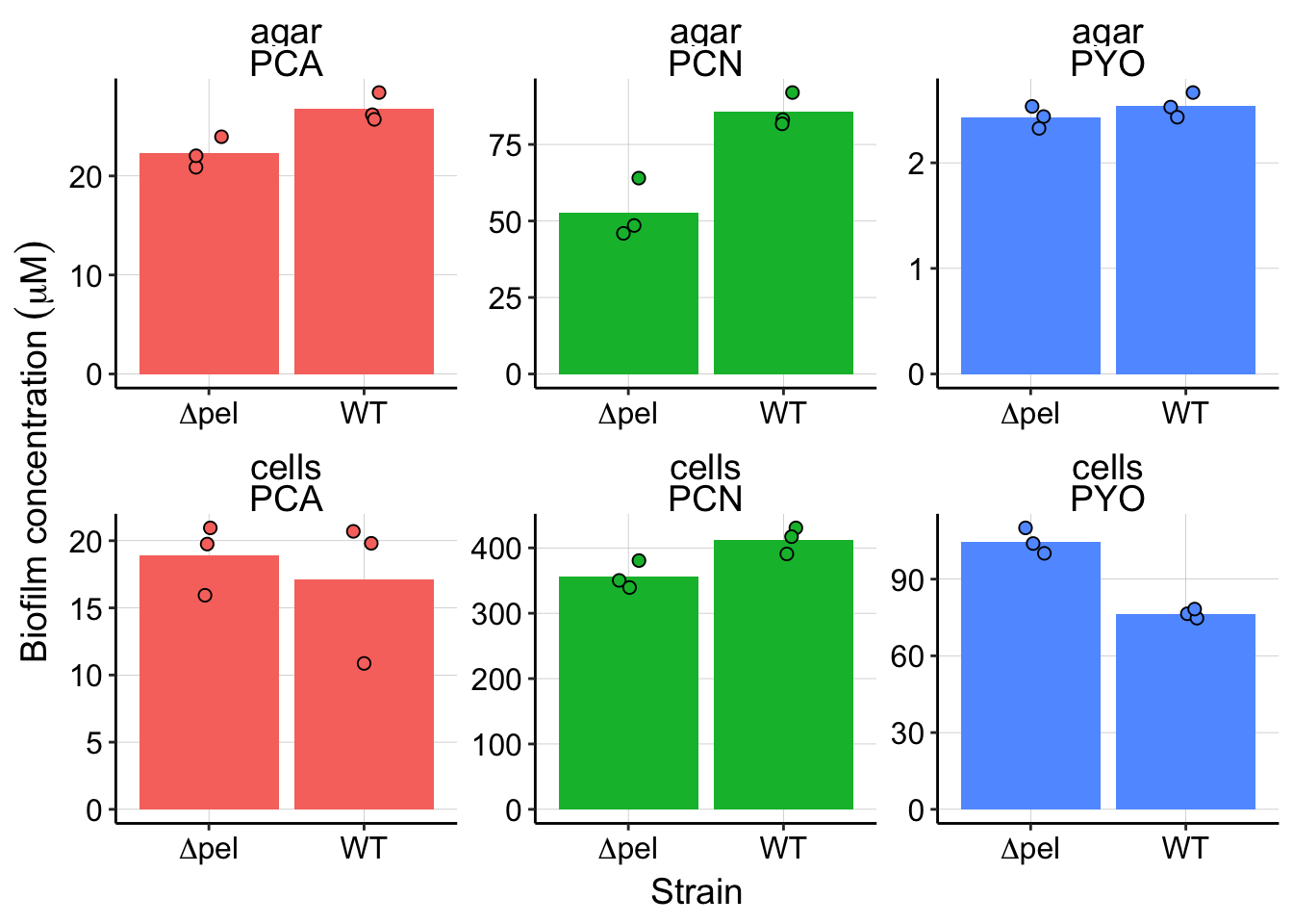 You can see that for each phenazine the concentration differs between the strains for both the cells aka biofilm and the agar. What we actually care about is the retention ratio, so let’s calculate and look at that.
# Split dataset by material
pel_extracts_means_agar <- pel_extracts_means %>% filter(material ==
"agar")
pel_extracts_means_biofilm <- pel_extracts_means %>% filter(material ==
"cells")
# Join agar and cell observations and calculate retention
# ratios = biofilm / agar
pel_extracts_means_join <- left_join(pel_extracts_means_biofilm,
pel_extracts_means_agar, by = c("strain", "replicate", "measured_phenazine"),
suffix = c("_from_biofilm", "_from_agar")) %>% mutate(retention_ratio = calcConc_from_biofilm/calcConc_from_agar) %>%
mutate(mean_retention_ratio = mean_from_biofilm/mean_from_agar)
# Plot Layout
plot_pel <- ggplot(pel_extracts_means_join, aes(x = strain, y = retention_ratio,
fill = measured_phenazine)) + geom_col(aes(y = mean_retention_ratio)) +
geom_jitter(width = 0.1, height = 0, shape = 21, size = 2) +
facet_wrap(~measured_phenazine, scales = "free")
# Styling
plot_pel_styled <- plot_pel + scale_x_discrete(breaks = c("WTpar",
"dPel"), labels = c("WT", expression(Delta * "pel")), limits = c("WTpar",
"dPel")) + labs(x = NULL, y = expression(Biofilm/Agar)) +
theme(axis.text.x = element_text(size = 14)) + guides(fill = F)
plot_pel_styled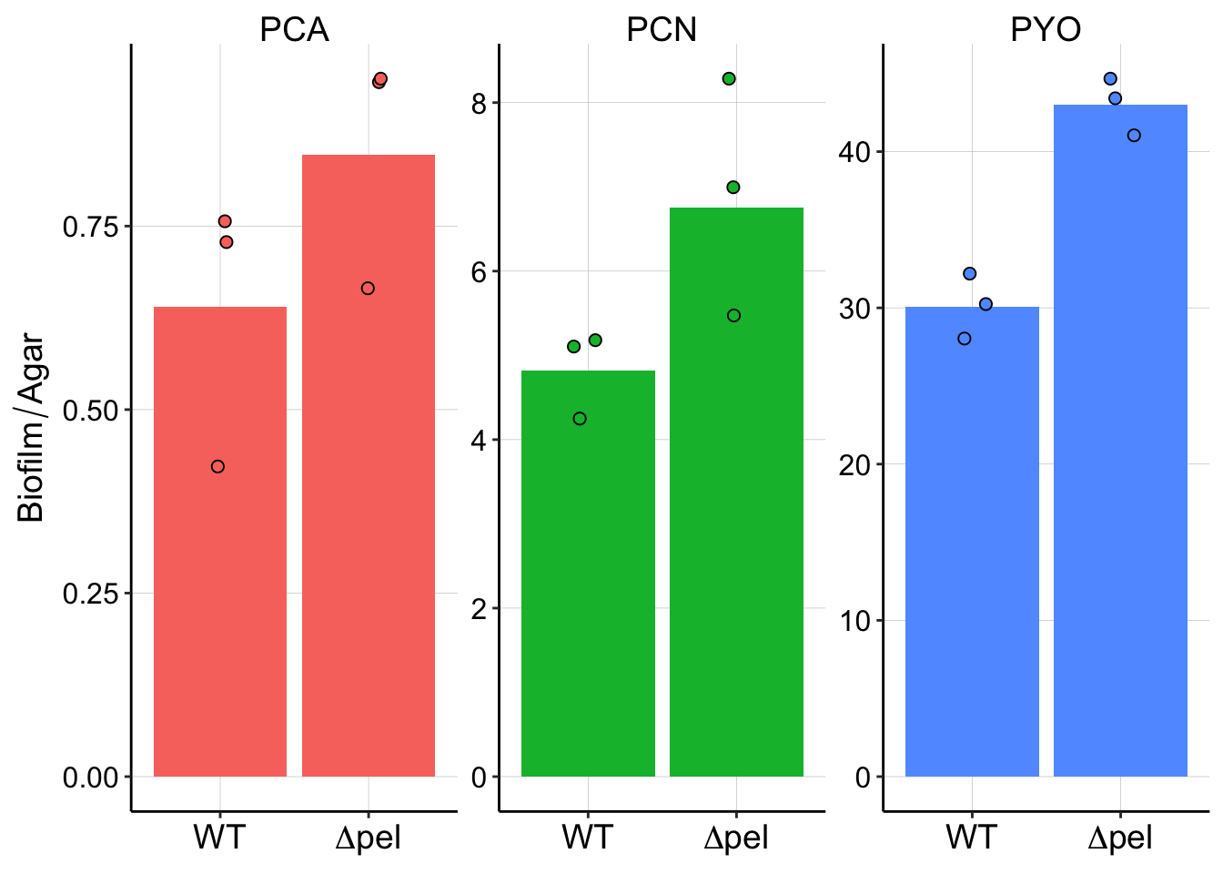 Cool, now we can see that indeed PYO may be more tightly retained in the pel mutant.
Panel B
Let’s read in the dnase dataset and look at the table:
dnase_extracts <- read_csv("../data/2018_10_08_HPLC_concentrations_df.csv",
    comment = "#") %>% filter(Strain == "WT" & Day == "D4") %>%
    group_by(Phenazine, Condition, Material) %>% mutate(mean = ifelse(Replicate ==
    1, mean(calcConc), NA))


dnase_extracts %>% kable() %>% kable_styling(bootstrap_options = c("striped",
    "hover", "condensed", "responsive"), full_width = F) %>%
scroll_box(height = "250px")| Phenazine | Strain | Condition | Replicate | Material | Day | RT | Area | Channel Name | Amount | calcConc | mean |
|---|---|---|---|---|---|---|---|---|---|---|---|
| PYO | WT | DNase | 1 | cells | D4 | 5.952 | 78120 | 313.0nm | 2.523 | 72.32600 | 71.055111 |
| PCA | WT | DNase | 1 | cells | D4 | 3.170 | 10966 | 364.0nm | 0.698 | 20.00933 | 17.601333 |
| PCN | WT | DNase | 1 | cells | D4 | 8.799 | 283489 | 364.0nm | 19.744 | 565.99467 | 567.934444 |
| PYO | WT | DNase | 1 | agar | D4 | 5.963 | 13770 | 313.0nm | 0.445 | 1.42400 | 1.163733 |
| PCA | WT | DNase | 1 | agar | D4 | 3.066 | 42599 | 364.0nm | 2.712 | 8.67840 | 7.740800 |
| PCN | WT | DNase | 1 | agar | D4 | 8.807 | 117981 | 364.0nm | 8.217 | 26.29440 | 24.491733 |
| PYO | WT | DNase | 2 | agar | D4 | 5.967 | 9463 | 313.0nm | 0.306 | 0.97920 | NA |
| PCA | WT | DNase | 2 | agar | D4 | 3.065 | 34587 | 364.0nm | 2.202 | 7.04640 | NA |
| PCN | WT | DNase | 2 | agar | D4 | 8.812 | 100344 | 364.0nm | 6.989 | 22.36480 | NA |
| PYO | WT | DNase | 3 | agar | D4 | 5.964 | 10533 | 313.0nm | 0.340 | 1.08800 | NA |
| PCA | WT | DNase | 3 | agar | D4 | 3.105 | 36801 | 364.0nm | 2.343 | 7.49760 | NA |
| PCN | WT | DNase | 3 | agar | D4 | 8.803 | 111355 | 364.0nm | 7.755 | 24.81600 | NA |
| PYO | WT | none | 1 | agar | D4 | 5.971 | 15508 | 313.0nm | 0.501 | 1.60320 | 1.349333 |
| PCA | WT | none | 1 | agar | D4 | 3.054 | 43066 | 364.0nm | 2.742 | 8.77440 | 8.238933 |
| PCN | WT | none | 1 | agar | D4 | 8.815 | 75035 | 364.0nm | 5.226 | 16.72320 | 22.126933 |
| PYO | WT | none | 2 | agar | D4 | 5.968 | 12382 | 313.0nm | 0.400 | 1.28000 | NA |
| PCA | WT | none | 2 | agar | D4 | 3.060 | 40419 | 364.0nm | 2.573 | 8.23360 | NA |
| PCN | WT | none | 2 | agar | D4 | 8.814 | 101441 | 364.0nm | 7.065 | 22.60800 | NA |
| PYO | WT | none | 3 | agar | D4 | 5.964 | 11287 | 313.0nm | 0.364 | 1.16480 | NA |
| PCA | WT | none | 3 | agar | D4 | 3.059 | 37847 | 364.0nm | 2.409 | 7.70880 | NA |
| PCN | WT | none | 3 | agar | D4 | 8.811 | 121366 | 364.0nm | 8.453 | 27.04960 | NA |
| PYO | WT | DNase | 2 | cells | D4 | 5.942 | 75064 | 313.0nm | 2.424 | 69.48800 | NA |
| PCA | WT | DNase | 2 | cells | D4 | 3.132 | 9362 | 364.0nm | 0.596 | 17.08533 | NA |
| PCN | WT | DNase | 2 | cells | D4 | 8.789 | 285936 | 364.0nm | 19.915 | 570.89667 | NA |
| PYO | WT | DNase | 3 | cells | D4 | 5.949 | 77070 | 313.0nm | 2.489 | 71.35133 | NA |
| PCA | WT | DNase | 3 | cells | D4 | 3.119 | 8611 | 364.0nm | 0.548 | 15.70933 | NA |
| PCN | WT | DNase | 3 | cells | D4 | 8.797 | 283951 | 364.0nm | 19.776 | 566.91200 | NA |
| PYO | WT | none | 1 | cells | D4 | 5.957 | 102908 | 313.0nm | 3.323 | 95.25933 | 88.847556 |
| PCA | WT | none | 1 | cells | D4 | 3.113 | 13782 | 364.0nm | 0.877 | 25.14067 | 20.324667 |
| PCN | WT | none | 1 | cells | D4 | 8.804 | 306236 | 364.0nm | 21.328 | 611.40267 | 614.231111 |
| PYO | WT | none | 2 | cells | D4 | 5.946 | 98479 | 313.0nm | 3.180 | 91.16000 | NA |
| PCA | WT | none | 2 | cells | D4 | 3.100 | 9417 | 364.0nm | 0.599 | 17.17133 | NA |
| PCN | WT | none | 2 | cells | D4 | 8.792 | 301514 | 364.0nm | 20.999 | 601.97133 | NA |
| PYO | WT | none | 3 | cells | D4 | 5.931 | 86539 | 313.0nm | 2.795 | 80.12333 | NA |
| PCA | WT | none | 3 | cells | D4 | 3.092 | 10222 | 364.0nm | 0.651 | 18.66200 | NA |
| PCN | WT | none | 3 | cells | D4 | 8.778 | 315202 | 364.0nm | 21.953 | 629.31933 | NA |
Now, let’s look at an overview of the experiment.
ggplot(dnase_extracts, aes(x = Condition, y = calcConc, fill = Phenazine)) +
geom_col(aes(y = mean)) + geom_jitter(width = 0.1, height = 0,
shape = 21, size = 2) + facet_wrap(Material ~ Phenazine,
scales = "free")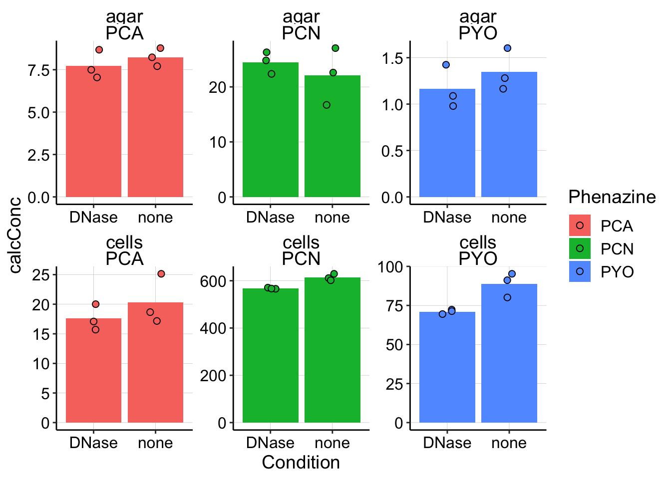 Here you can see that the agar concentrations between the Dnase treated and untreated don’t differ meaningfully, but the cell/biofilm concentrations might. So, let’s ignore the agar concentrations for now. It’s also important to note that by calculating a ratio as we did above for pel we do risk amplifying meaningless differences by dividing large numbers by small numbers.
Here’s the biofilm only:
# Plot layout
dnase_plot <- ggplot(dnase_extracts %>% filter(Material == "cells"),
aes(x = Condition, y = calcConc, fill = Phenazine)) + geom_col(aes(y = mean)) +
geom_jitter(width = 0.1, height = 0, shape = 21, size = 2) +
facet_wrap(~Phenazine, scales = "free")
# Plot styling
dnase_plot_styled <- dnase_plot + labs(x = NULL, y = expression("Biofilm concentration" ~
(mu * M))) + scale_x_discrete(limits = c("none", "DNase")) +
guides(fill = F) + theme(axis.text.x = element_text(size = 14))
dnase_plot_styled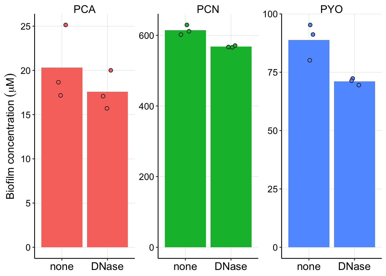 So there may be a difference for PYO and PCN, but it’s not dramatic.
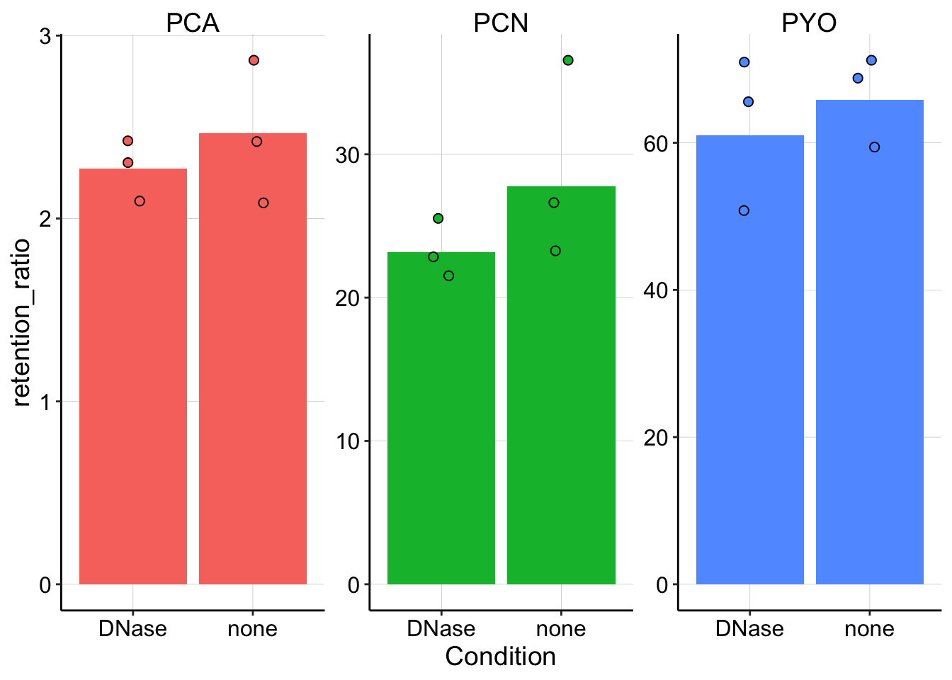
Here’s the retention ratios just for comparison:
# Split dataset by material
dnase_extracts_agar <- dnase_extracts %>% filter(Material ==
    "agar")

dnase_extracts_biofilm <- dnase_extracts %>% filter(Material ==
    "cells")

# Join agar and cell observations and calculate retention
# ratios = biofilm / agar
dnase_extracts_join <- left_join(dnase_extracts_biofilm, dnase_extracts_agar,
    by = c("Strain", "Replicate", "Phenazine", "Condition", "Day"),
    suffix = c("_from_biofilm", "_from_agar")) %>% mutate(retention_ratio = calcConc_from_biofilm/calcConc_from_agar) %>%
    mutate(mean_retention_ratio = mean_from_biofilm/mean_from_agar)

# Plot
ggplot(dnase_extracts_join, aes(x = Condition, y = retention_ratio,
    fill = Phenazine)) + geom_col(aes(y = mean_retention_ratio)) +
    geom_jitter(width = 0.1, height = 0, shape = 21, size = 2) +
    facet_wrap(~Phenazine, scales = "free") + guides(fill = F)