Note the YAML contains specifications for a github document and html. The best way to deal with this is to knit them separately from the knit menu. Otherwise the html has blurry plots and tends to delete the md cached plots unless you tell it to cache everything!

library(tidyverse)
library(cowplot)
library(broom) 
library(modelr) 
library(viridis)

knitr::opts_knit$set(root.dir = '/Users/scottsaunders/git/labwork/Figures/draft1/')
knitr::opts_chunk$set(tidy.opts=list(width.cutoff=60),tidy=TRUE, echo = TRUE, message=FALSE, warning=FALSE, fig.align="center")

theme_1 <- function () { 
    theme_classic() %+replace% 
        theme(
          axis.text = element_text( size=12),
          axis.title=element_text(size=14),
          strip.text = element_text(size = 14),
          strip.background = element_rect(color='white'),
          legend.title=element_text(size=14),
          legend.text=element_text(size=12),
          panel.grid.major = element_line(color='grey',size=0.1)
        )
}

theme_set(theme_1())

Let’s read in the data from a cleaned csv file and remove the blank and standard samples.

df_pel <- read_csv("../data/2018_10_30_HPLC_concentrations_df.csv", 
    comment = "#")

pel_panel <- df_pel %>% filter(strain %in% c("WTpar", "dPel")) %>% 
    filter(material == "cells") %>% ggplot(aes(x = strain, y = calcConc, 
    fill = measured_phenazine)) + geom_jitter(width = 0.1, height = 0, 
    shape = 21, size = 2) + facet_wrap(~measured_phenazine, scales = "free", 
    ncol = 1, strip.position = "right") + ylim(0, NA) + scale_x_discrete(breaks = c("dPel", 
    "WTpar"), labels = c(expression(Delta * "pel"), "WT")) + 
    labs(x = "Strain", y = expression("Biofilm calculated concentration (" ~ 
        mu * "M)")) + guides(fill = F)
pel_panel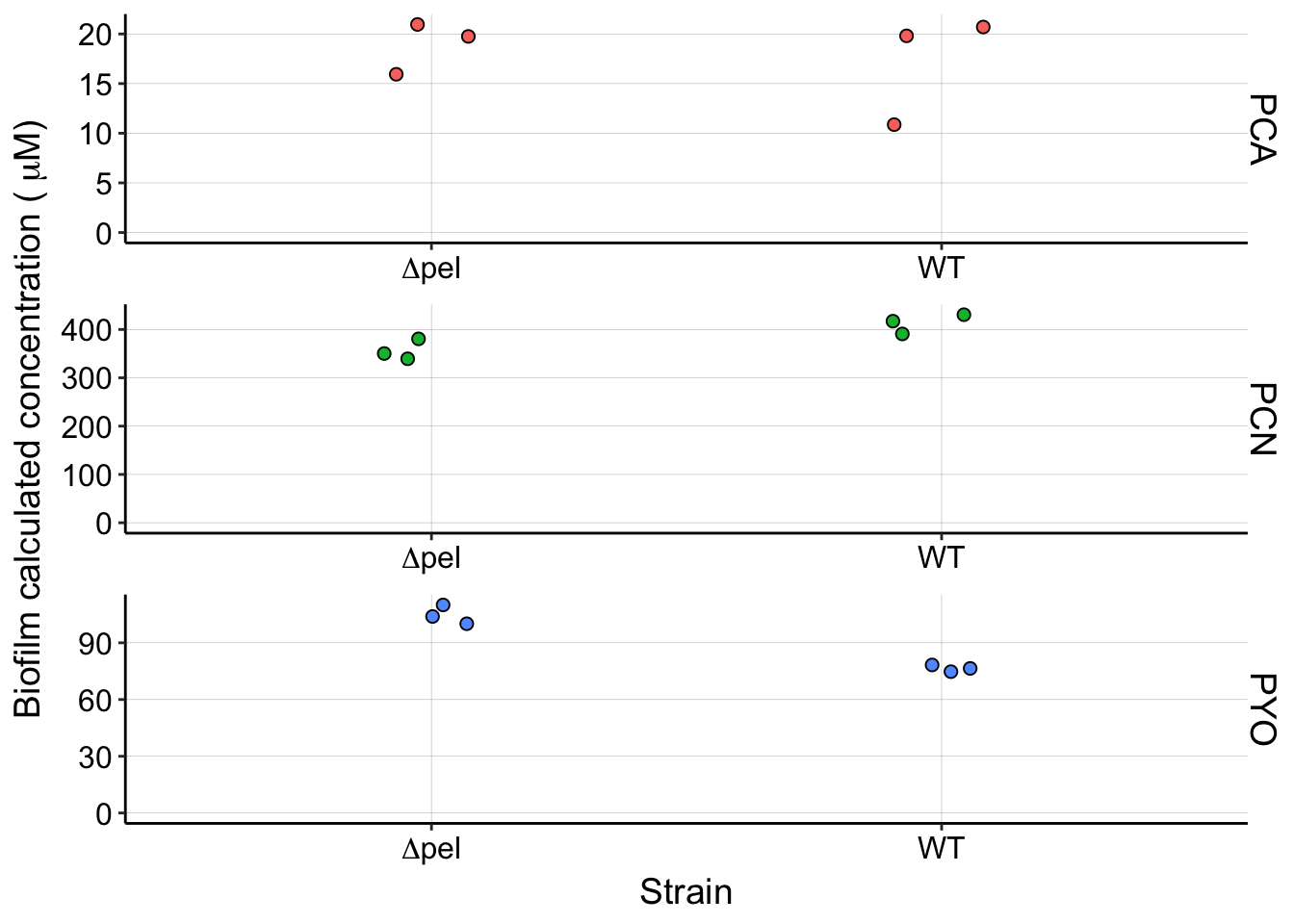

df_dnase <- read_csv("../data/2018_10_08_HPLC_concentrations_df.csv", 
    comment = "#")

dnase_panel <- df_dnase %>% filter(Strain == "WT" & Material == 
    "cells") %>% ggplot(aes(x = Condition, y = calcConc, fill = Phenazine)) + 
    geom_jitter(width = 0.1, height = 0, shape = 21, size = 2) + 
    facet_wrap(Phenazine ~ ., scales = "free", ncol = 1, strip.position = "right") + 
    ylim(0, NA) + scale_x_discrete(breaks = c("DNase", "none"), 
    labels = c("+", "-")) + labs(x = "DNase treatment", y = expression("Biofilm calculated concentration (" ~ 
    mu * "M)")) + guides(fill = F)

dnase_panel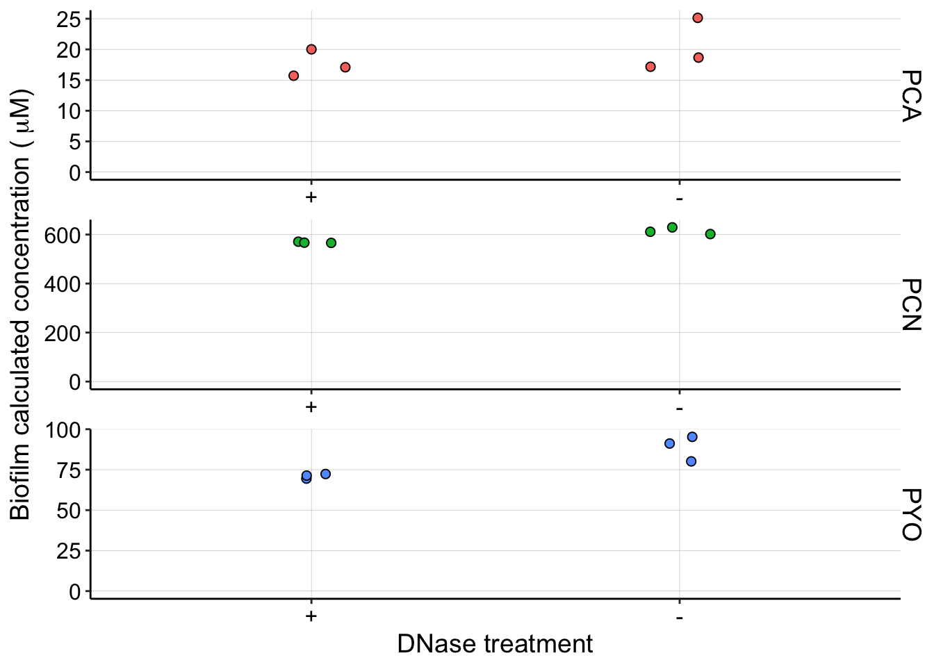

dnasePel <- plot_grid(pel_panel, dnase_panel, ncol = 2, labels = c("A", 
    "B"), align = "hv", axis = "tblr", scale = 0.9)

dnasePel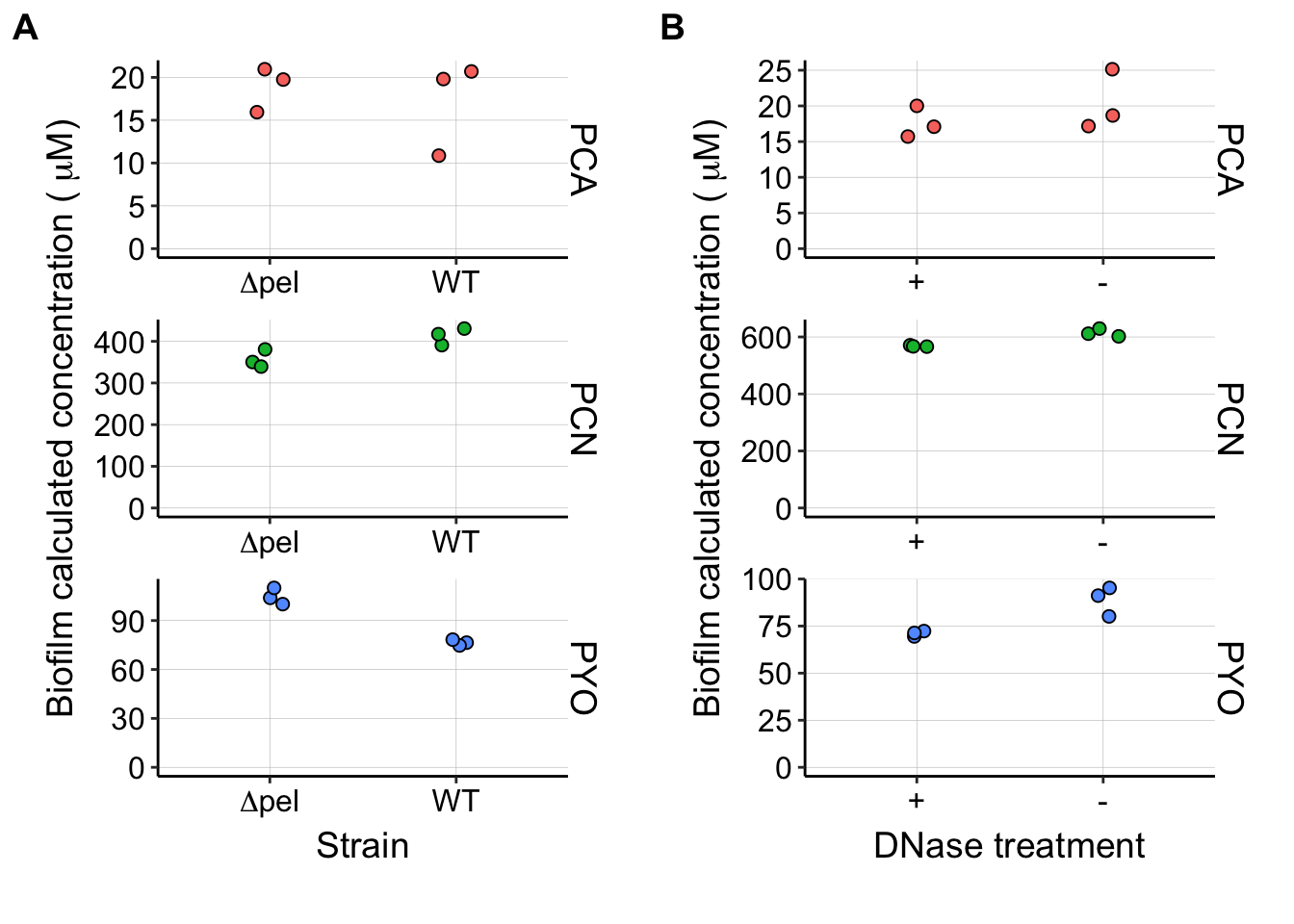

# ggsave('fig2ab.pdf',dnasePel, height = 8 , width = 6)