ctDNA calibration curve

Let’s go ahead and read in the data and metadata and combine into a nice long form to work with.

cal_data <- read_csv("../pr_data/07_23_19_ctDNA_calcurve_toto1_data.csv") %>% 
    gather(key = "Well", value = "FluorInt", -Wavelength)

cal_meta <- read_csv("../pr_data/07_23_19_ctDNA_calcurve_toto1_well_metadata.csv", 
    skip = 1, col_types = "cd")

cal_df <- left_join(cal_data, cal_meta, by = "Well")

tail(cal_df) %>% kable() %>% kable_styling()

Wavelength	Well	FluorInt	DNA_conc
600	C6	211	0.0076294
605	C6	189	0.0076294
610	C6	172	0.0076294
615	C6	155	0.0076294
620	C6	141	0.0076294
625	C6	134	0.0076294

Here’s what all the data look like:

ggplot(cal_df, aes(x = Wavelength, y = FluorInt, color = Well)) + 
    geom_path() + scale_color_discrete()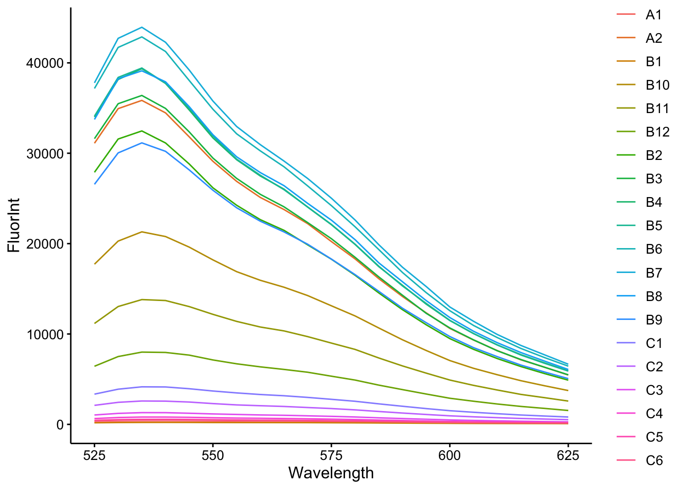

So you can see that we have a wide variety of intensities (despite the same amount of dye), but clearly the emission is the same shape and peak is at 535. Let’s just look at the ctDNA concentration vs. Fluorescence Intensity at 535nm:

ggplot(cal_df %>% filter(Wavelength == 535), aes(x = DNA_conc, 
    y = FluorInt)) + geom_point()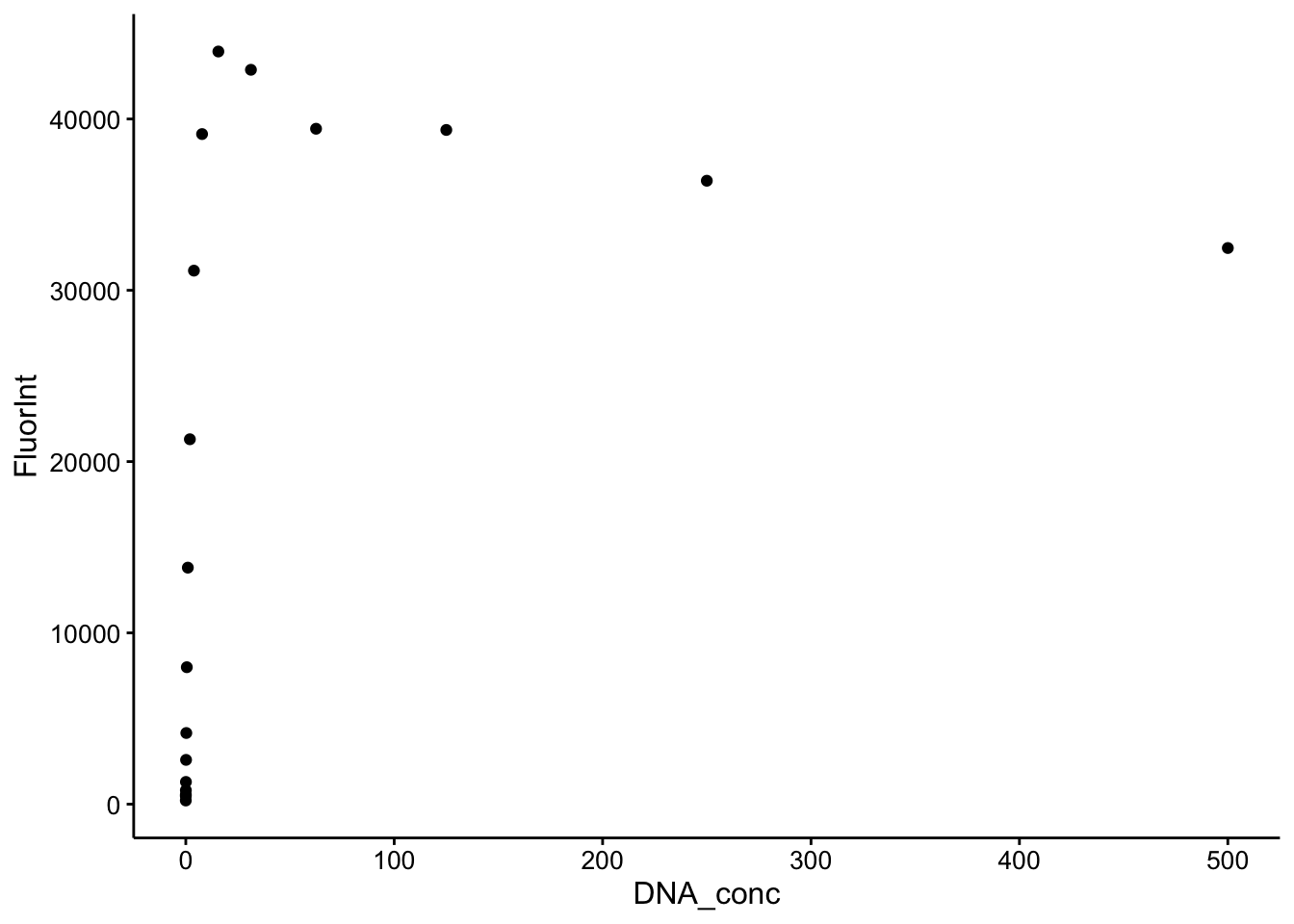

ggplot(cal_df %>% filter(Wavelength == 535) %>% filter(DNA_conc < 
    5), aes(x = DNA_conc, y = FluorInt)) + geom_point()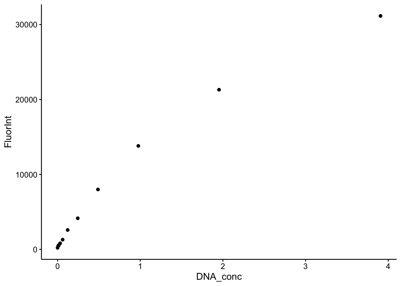

So the higher values of the DNA definitely saturate the Dye (top), but zooming in (bottom) shows a nice binding curve like response. It’s not perfectly linear at this scale, but the important part is that more DNA yields more dye fluorescence in a reasonable manner.

I’ve taken the liberty of glancing ahead at the colony fluorescence values. They span ~5000 to 15000 fluorescence units, so let’s zoom in a little further and flip the axes to see what our calibration curve looks like in that region.

ggplot(cal_df %>% filter(Wavelength == 535) %>% filter(DNA_conc < 
    1), aes(x = FluorInt, y = DNA_conc)) + geom_smooth(method = "lm") + 
    geom_point(shape = 21)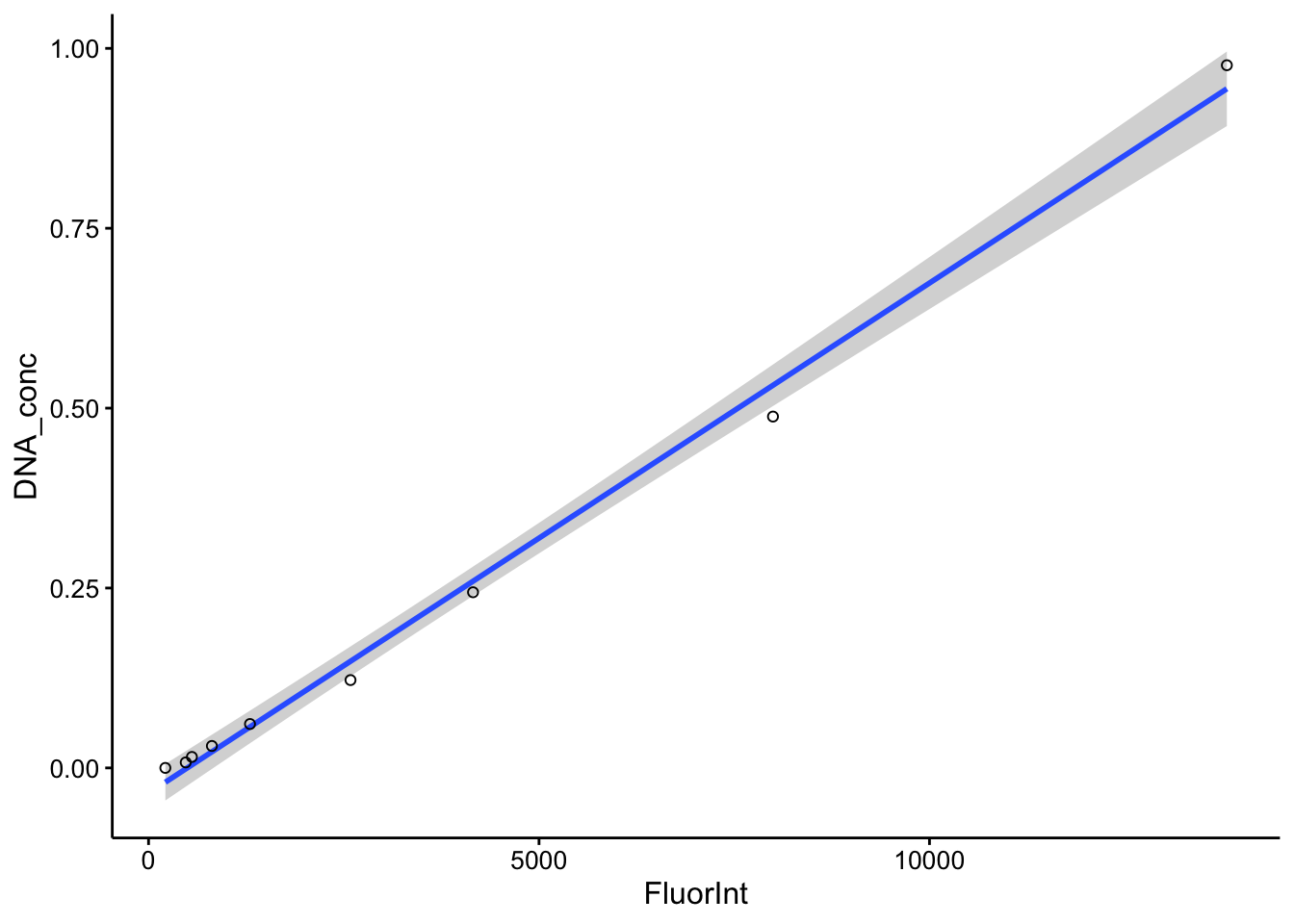

Not bad…it’s a little sparse in this region and the response probably isn’t truly linear, but the linear model will allow us to make a reasonable extrapolation between the datapoints. If we were feeling fancy we could probably fit an actual binding curve to this data and use that as the calibration curve model.

Anyway, here’s the model we will actually use:

cal_model <- lm(DNA_conc ~ FluorInt, data = cal_df %>% filter(Wavelength == 
    535) %>% filter(DNA_conc < 1))

summary(cal_model)

## 
## Call:
## lm(formula = DNA_conc ~ FluorInt, data = cal_df %>% filter(Wavelength == 
##     535) %>% filter(DNA_conc < 1))
## 
## Residuals:
##       Min        1Q    Median        3Q       Max 
## -0.043478 -0.015304  0.008152  0.011042  0.032752 
## 
## Coefficients:
##               Estimate Std. Error t value Pr(>|t|)    
## (Intercept) -3.513e-02  1.100e-02  -3.193   0.0152 *  
## FluorInt     7.090e-05  1.967e-06  36.038 3.29e-09 ***
## ---
## Signif. codes:  0 '***' 0.001 '**' 0.01 '*' 0.05 '.' 0.1 ' ' 1
## 
## Residual standard error: 0.02553 on 7 degrees of freedom
## Multiple R-squared:  0.9946, Adjusted R-squared:  0.9939 
## F-statistic:  1299 on 1 and 7 DF,  p-value: 3.29e-09

So the linear model fits reasonably well even though it’s probably wrong. Let’s move forward using this despite its imperfections, it should allow us to make a reasonable statement about the eDNA concentration in terms of the ctDNA equivalent.

WT colony measurements

Ok, now the exciting part. Let’s take a look at the colony data in the same format:

wt_data <- read_csv("../pr_data/07_23_19_WT_colonies_toto1_data.csv") %>% 
    gather(key = "Well", value = "FluorInt", -Wavelength)

wt_meta <- read_csv("../pr_data/07_23_19_WT_colony_toto1_well_metadata.csv")

wt_df <- left_join(wt_data, wt_meta, by = "Well")

tail(wt_df) %>% kable() %>% kable_styling()

Wavelength	Well	FluorInt	Condition	Colony_number	Replicate
600	G6	3076	TOTO	6	3
605	G6	2753	TOTO	6	3
610	G6	2435	TOTO	6	3
615	G6	2179	TOTO	6	3
620	G6	1958	TOTO	6	3
625	G6	1744	TOTO	6	3

ggplot(wt_df %>% filter(Wavelength == 535), aes(x = Colony_number, 
    y = FluorInt, shape = Condition)) + geom_point() + ylim(0, 
    15000)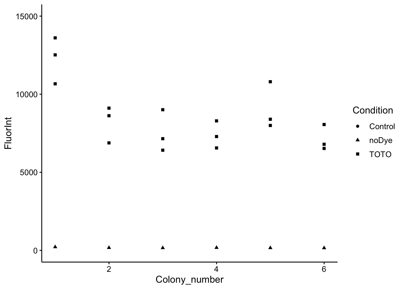

Ok, so we can learn a vew things from this. First, there is some biological variation between the colonies, but overall they’re in a pretty tight window. The other thing we can see is that there is significant technical variation within each colony from the technical triplicates. This probably makes sense as the bit of biofilm that gets resuspended in each well may be quite different. Lastly, the background fluorescence is really negligible. Overall, I think these data look pretty good!

Prediction of eDNA concentration

Now let’s try to convert those fluorescence intensity values into predictions for the amount of eDNA in each colony biofilm.

We can use the linear model from the calf thymus calibration curve to add predictions from the WT colony data, but that only gives us a value in terms of ug / mL of ctDNA in the well. We really want to get to uM bp dsDNA.

So first we are going to multiply by 4 to get from the concentration in the well to the concentration of eDNA in the biofilm suspension tube. Then we can convert into the concentration in the biofilm by multiplying by the dilution factor 800uL / 60uL.

Lastly, we need to go from ug / mL to uM by using a conversion factor from NEB which is that 50 ug / mL DNA is equivalent to 150uM dsDNA bp, so we multiply by 150 / 50. That gives us a dataframe that looks like this:

wt_preds <- wt_df %>% filter(Wavelength == 535) %>% add_predictions(cal_model) %>% 
    mutate(eDNA_ug_mL = pred * 4 * 800/60) %>% mutate(eDNA_dsDNA_uM = eDNA_ug_mL * 
    150/50)

# write_csv(wt_preds,
# '07_23_19_wt_TOTO_calCurve_estimates.csv')

tail(wt_preds) %>% kable() %>% kable_styling()

Wavelength	Well	FluorInt	Condition	Colony_number	Replicate	pred	eDNA_ug_mL	eDNA_dsDNA_uM
535	G1	13607	TOTO	1	3	0.9295607	49.57657	148.72971
535	G2	8622	TOTO	2	3	0.5761404	30.72749	92.18247
535	G3	7151	TOTO	3	3	0.4718513	25.16540	75.49621
535	G4	8291	TOTO	4	3	0.5526736	29.47593	88.42778
535	G5	7998	TOTO	5	3	0.5319009	28.36805	85.10414
535	G6	8059	TOTO	6	3	0.5362256	28.59870	85.79609

So now we can view our WT colony measurements in terms of an estimated uM dsDNA bp:

ggplot(wt_preds, aes(x = Colony_number, y = eDNA_dsDNA_uM, shape = Condition)) + 
    geom_point() + ylim(0, 200) + guides(shape = "none")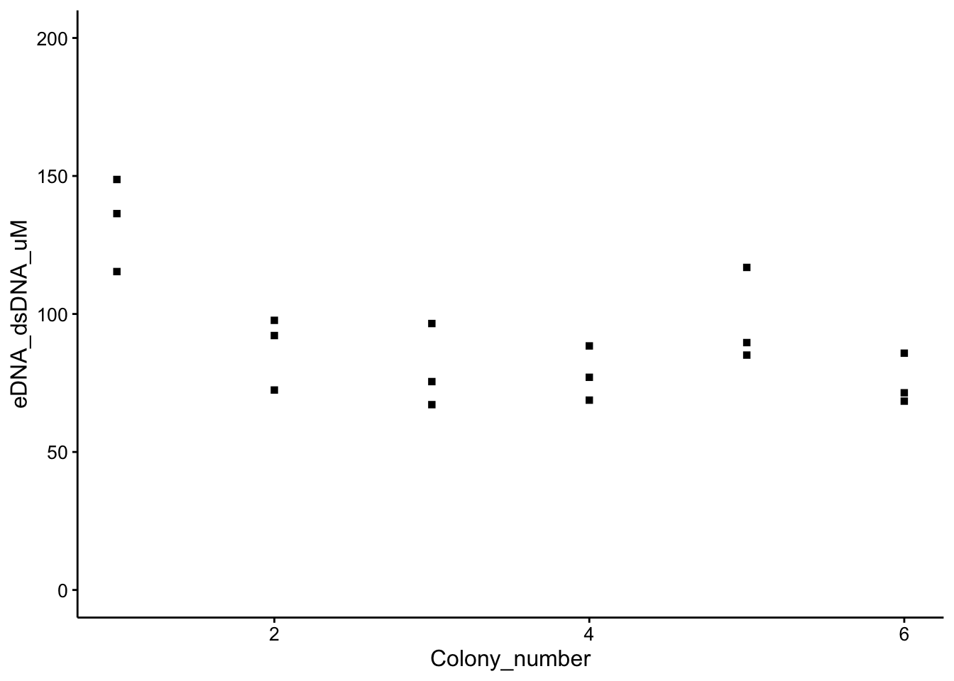

We can view all these measurements together with boxplot stats:

ggplot(wt_preds %>% filter(Condition == "TOTO"), aes(x = Condition, 
    y = eDNA_dsDNA_uM)) + geom_boxplot() + geom_jitter(shape = 21) + 
    ylim(0, 200)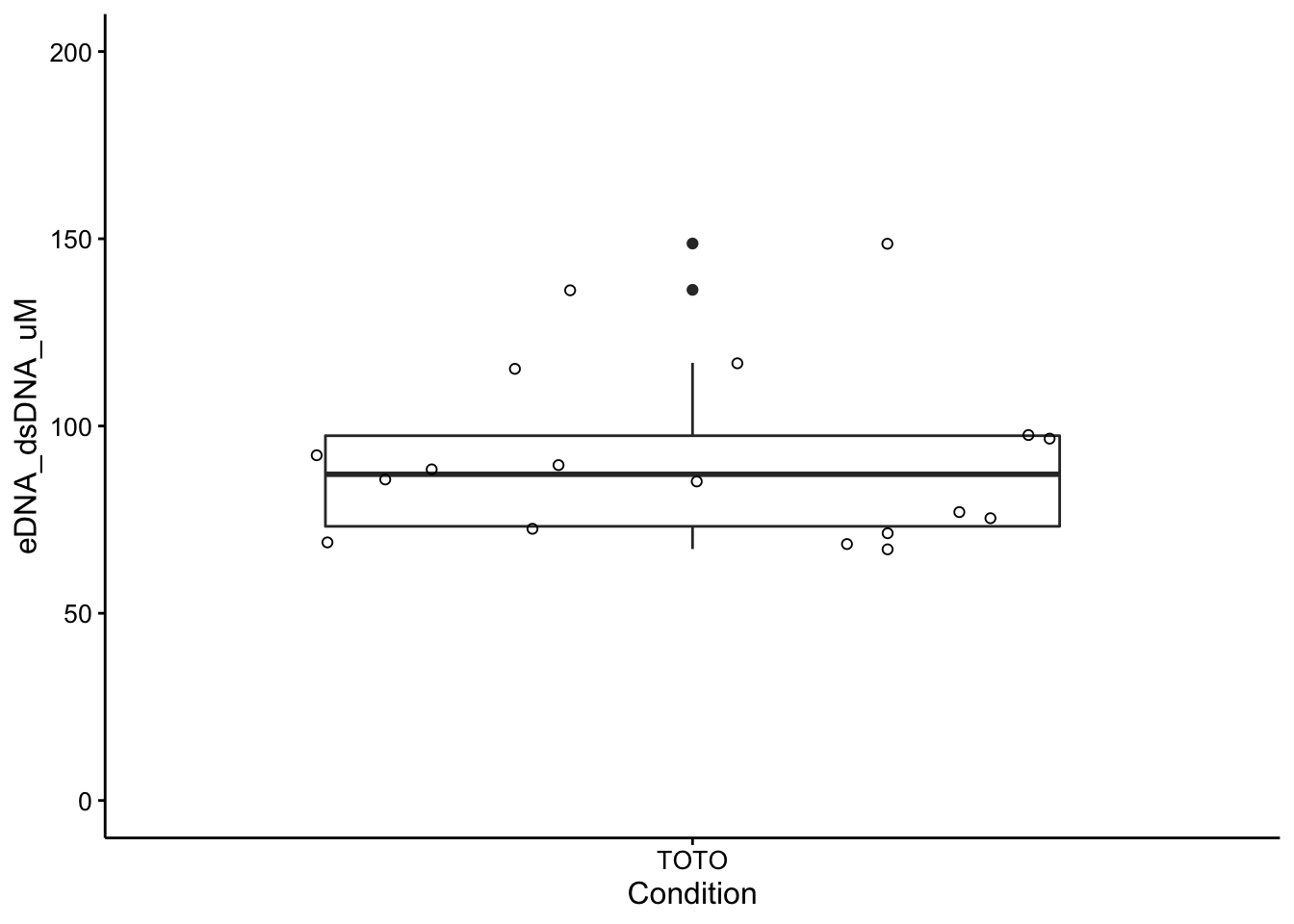

And if we take the mean value of each colony we get these numbers:

wt_means <- wt_preds %>% filter(Condition == "TOTO") %>% group_by(Colony_number) %>% 
    summarise(mean_eDNA = mean(eDNA_dsDNA_uM))

wt_means %>% kable() %>% kable_styling()

Colony_number	mean_eDNA
1	133.48408
2	87.44090
3	79.72733
4	78.09009
5	97.20007
6	75.22019

Finally taking the mean of those biological replicates gives a mean eDNA concentration of 91.860442 uM dsDNA bp.