Note the YAML contains specifications for a github document and html. The best way to deal with this is to knit them separately from the knit menu. Otherwise the html has blurry plots and tends to delete the md cached plots unless you tell it to cache everything!

library(tidyverse)
library(cowplot)
library(broom) 
library(modelr) 
library(viridis)

knitr::opts_knit$set(root.dir = '/Users/scottsaunders/git/labwork/HPLC/analysis/')
knitr::opts_chunk$set(tidy.opts=list(width.cutoff=60),tidy=TRUE, echo = TRUE, message=FALSE, warning=FALSE, fig.align="center")

theme_set(theme_bw())

Let’s read in the data from a cleaned csv file and remove the blank and standard samples.

df_wBlankStds <- read_csv("../data/2018_10_30_coloniesHPLCamounts.csv", 
    comment = "#")

head(df_wBlankStds)

## # A tibble: 6 x 10
##   measured_phenaz… strain amount_added added_phenazine material replicate
##   <chr>            <chr>  <chr>        <chr>           <chr>        <int>
## 1 PCA              dPHZs… 0.1uM        PCA             cells            2
## 2 PCA              dPHZs… 1uM          PCA             cells            2
## 3 PCA              dPHZs… 10uM         PCA             cells            2
## 4 PCA              dPHZs… 50uM         PCA             cells            2
## 5 PCA              dPHZs… 100uM        PCA             cells            2
## 6 PCA              dPHZs… 200uM        PCA             cells            2
## # ... with 4 more variables: RT <dbl>, Area <int>, `Channel Name` <chr>,
## #   Amount <dbl>

# Remove blanks and standards and calculate volume corrected
# concentration
df_amounts <- df_wBlankStds %>% filter(strain != "blank" & strain != 
    "PHZstd") %>% mutate(calcConc = ifelse(material == "cells", 
    Amount * 2 * (860/60), Amount * 2 * (8/5)))

Now let’s look at the dPHZstar experiment where we added different phenazines at different levels.

df_dPHZstar <- df_amounts %>% filter(strain == "dPHZstar") %>% 
    mutate(added_phz_int = as.integer(str_extract(amount_added, 
        "^[0-9]+")))

head(df_dPHZstar)

## # A tibble: 6 x 12
##   measured_phenaz… strain amount_added added_phenazine material replicate
##   <chr>            <chr>  <chr>        <chr>           <chr>        <int>
## 1 PCA              dPHZs… 0.1uM        PCA             cells            2
## 2 PCA              dPHZs… 1uM          PCA             cells            2
## 3 PCA              dPHZs… 10uM         PCA             cells            2
## 4 PCA              dPHZs… 50uM         PCA             cells            2
## 5 PCA              dPHZs… 100uM        PCA             cells            2
## 6 PCA              dPHZs… 200uM        PCA             cells            2
## # ... with 6 more variables: RT <dbl>, Area <int>, `Channel Name` <chr>,
## #   Amount <dbl>, calcConc <dbl>, added_phz_int <int>

Cool, now let’s plot some things.

ggplot(df_dPHZstar, aes(x = added_phz_int, y = calcConc, color = material)) + 
    geom_point() + facet_grid(added_phenazine ~ measured_phenazine, 
    scales = "free")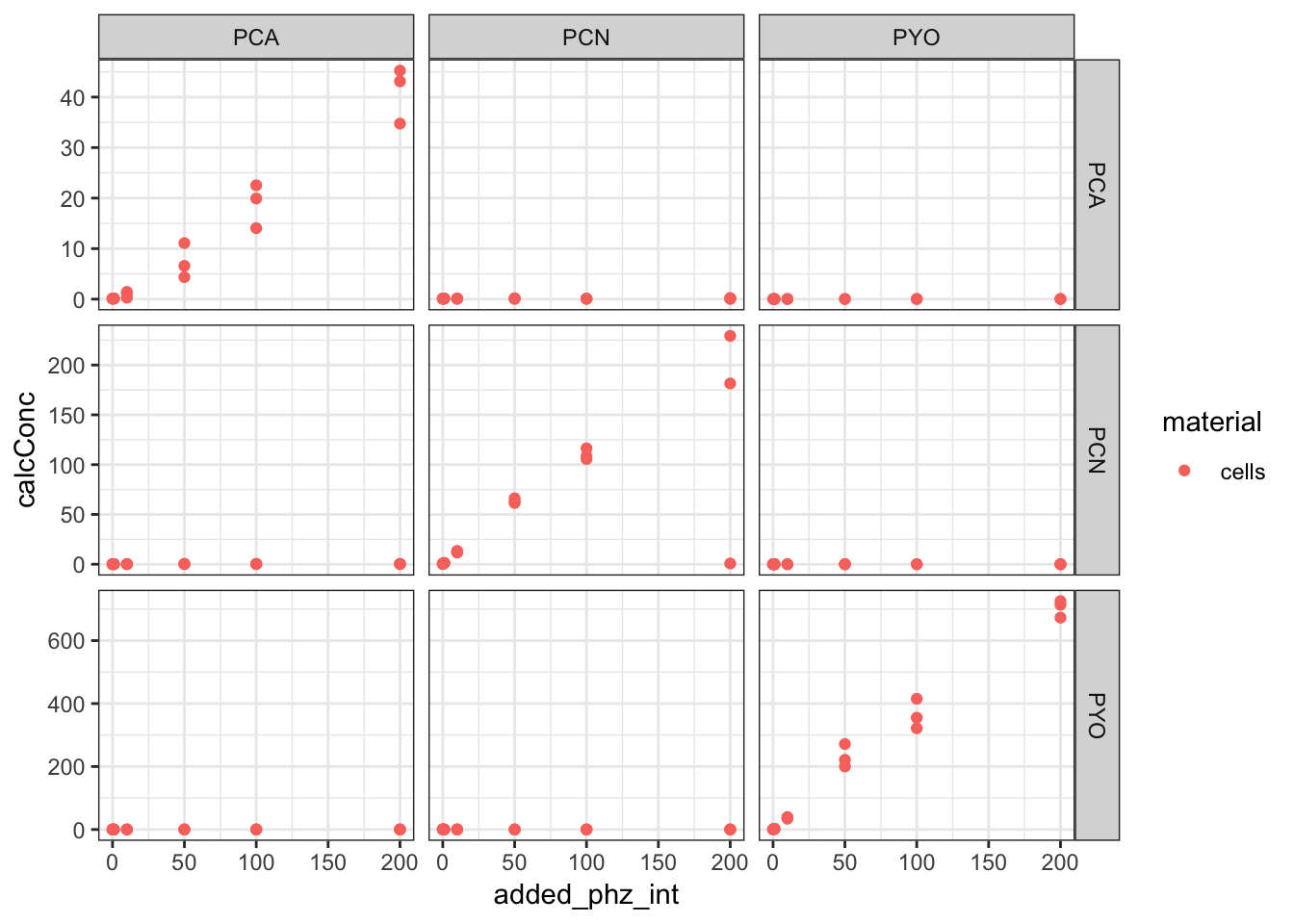

So from this overview, we can see that we only detect significant levels of phenazine in the dPHZstar mutant when we add that specific phenazine - for example, PCA is only detected significantly when we add PCA. So let’s just consider those samples. Also, we only have cell material for these samples, so we don’t need to worry about agar.

df_dPHZstar_match <- df_dPHZstar %>% filter(measured_phenazine == 
    added_phenazine)

ggplot(df_dPHZstar_match, aes(x = added_phz_int, y = calcConc, 
    color = measured_phenazine)) + geom_point() + facet_wrap(~measured_phenazine, 
    scales = "free")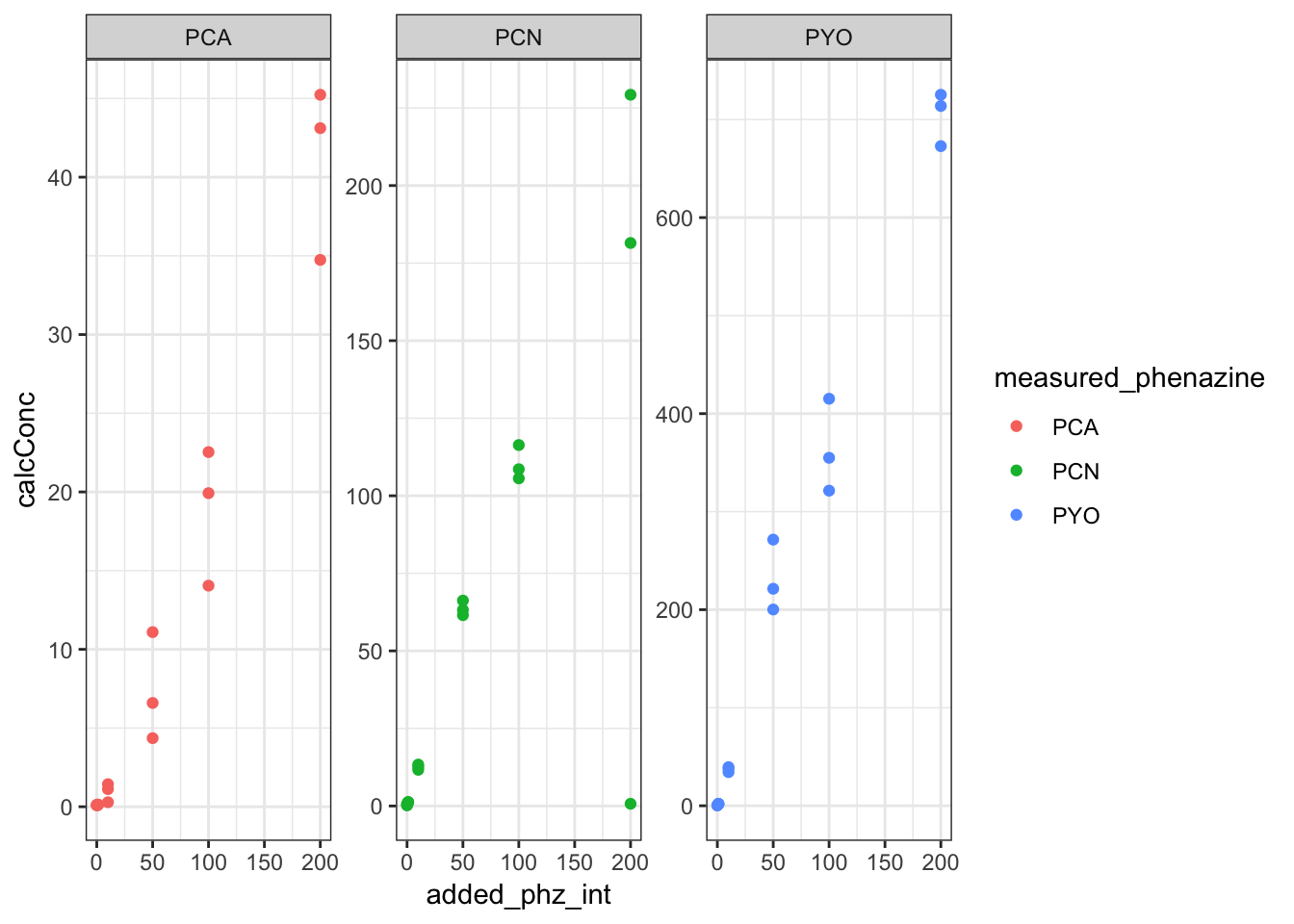

ggplot(df_dPHZstar_match, aes(x = added_phz_int, y = calcConc, 
    color = measured_phenazine, shape = factor(replicate))) + 
    geom_point() + geom_line() + geom_abline(slope = 1)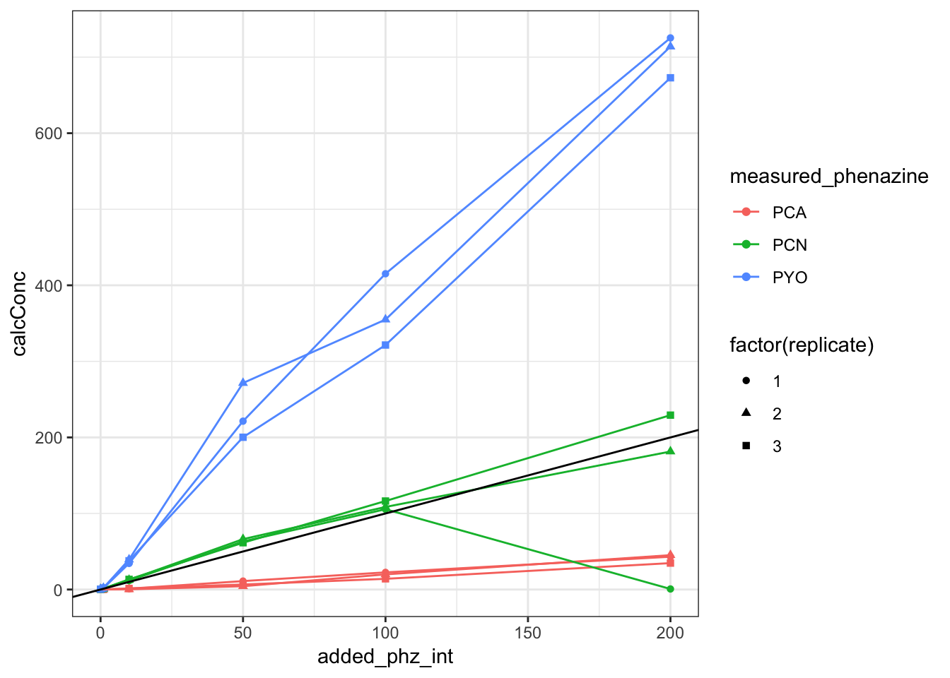

ggplot(df_dPHZstar_match, aes(x = added_phz_int, y = calcConc - 
    added_phz_int, color = measured_phenazine, shape = factor(replicate))) + 
    geom_point() + geom_line() + geom_abline(slope = 0)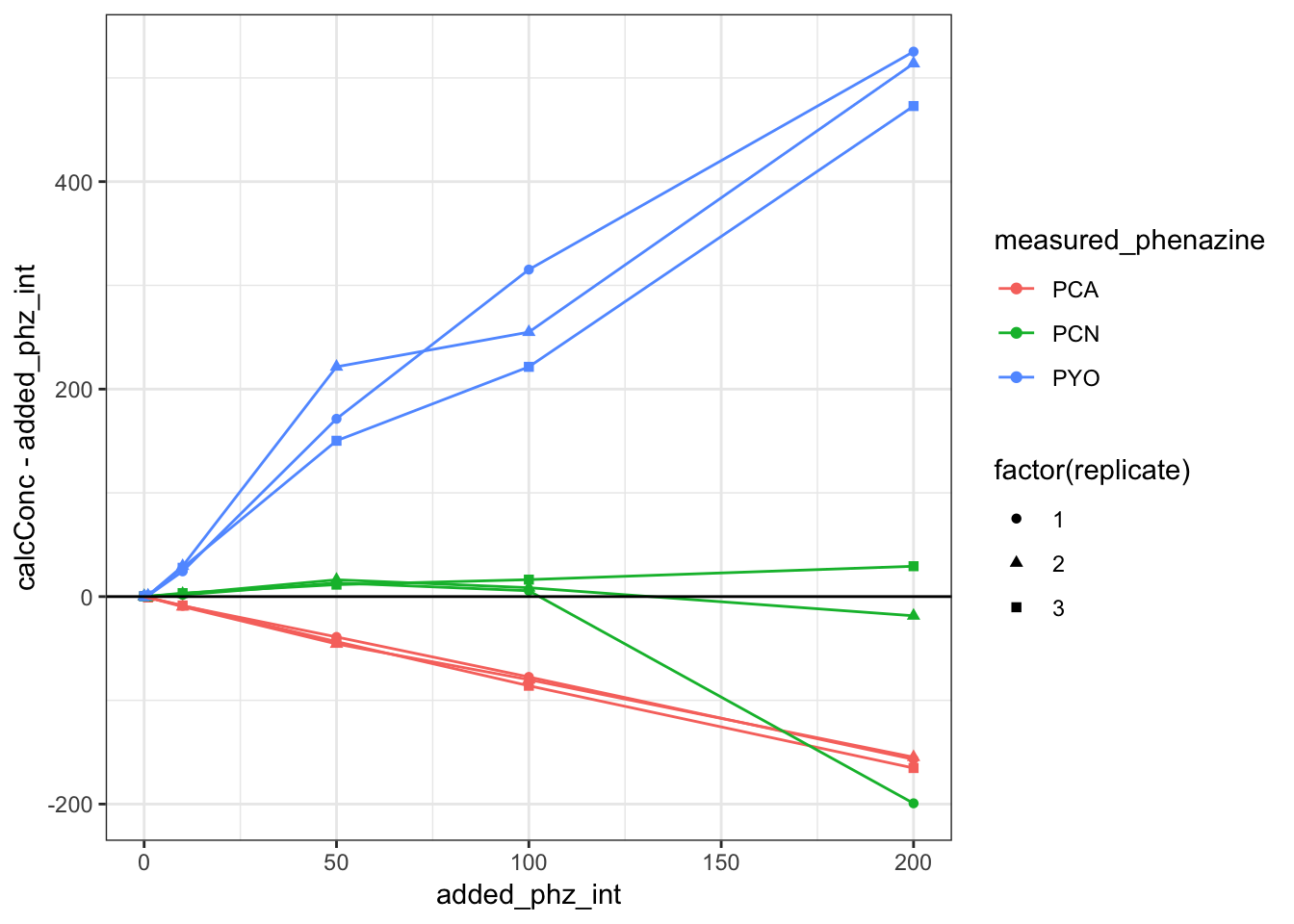

You can see that there’s one PCN sample (200uM rep1) that is unusually low. Apparently the RT drifted slightly earlier and the integration algorithm missed it. I manually looked at the peak and it seems to be about 7.7uM (uncorrected) which is right in line with the other replciates. Let’s move on for now, before thinking about reprocessing the whole dataset.

PCA being so low could either be due to the relevant volume actually being much less, for example, just the volume of the ECM not the whole biofilm. Or it could be that PCA actually has some affinity for the agar. Megan B.’s ideas.

Now let’s look at the other mutants

df_parsek <- df_amounts %>% filter(strain %in% c("WTpar", "dPel", 
    "pBadPel"))

ggplot(df_parsek %>% filter(strain != "pBadPel"), aes(x = strain, 
    y = calcConc, color = measured_phenazine)) + geom_point() + 
    facet_grid(measured_phenazine ~ material, scales = "free") + 
    ylim(0, NA) + theme(strip.background = element_rect(fill = "white"))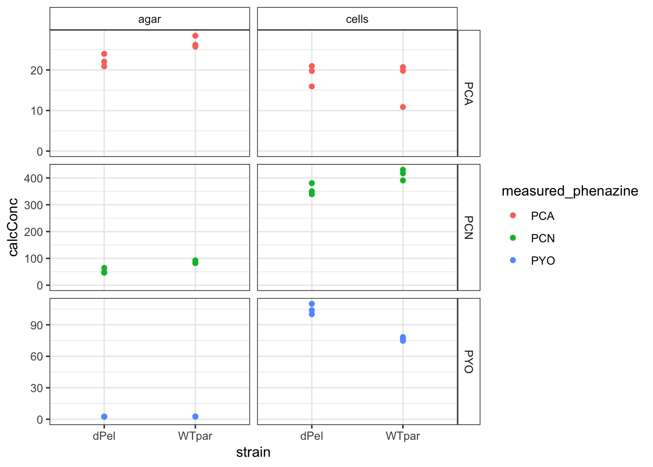

ggplot(df_parsek %>% filter(measured_phenazine == "PYO"), aes(x = strain, 
    y = calcConc, color = measured_phenazine)) + geom_point() + 
    facet_wrap(~material, scales = "free") + ylim(0, NA) + theme(strip.background = element_rect(fill = "white"))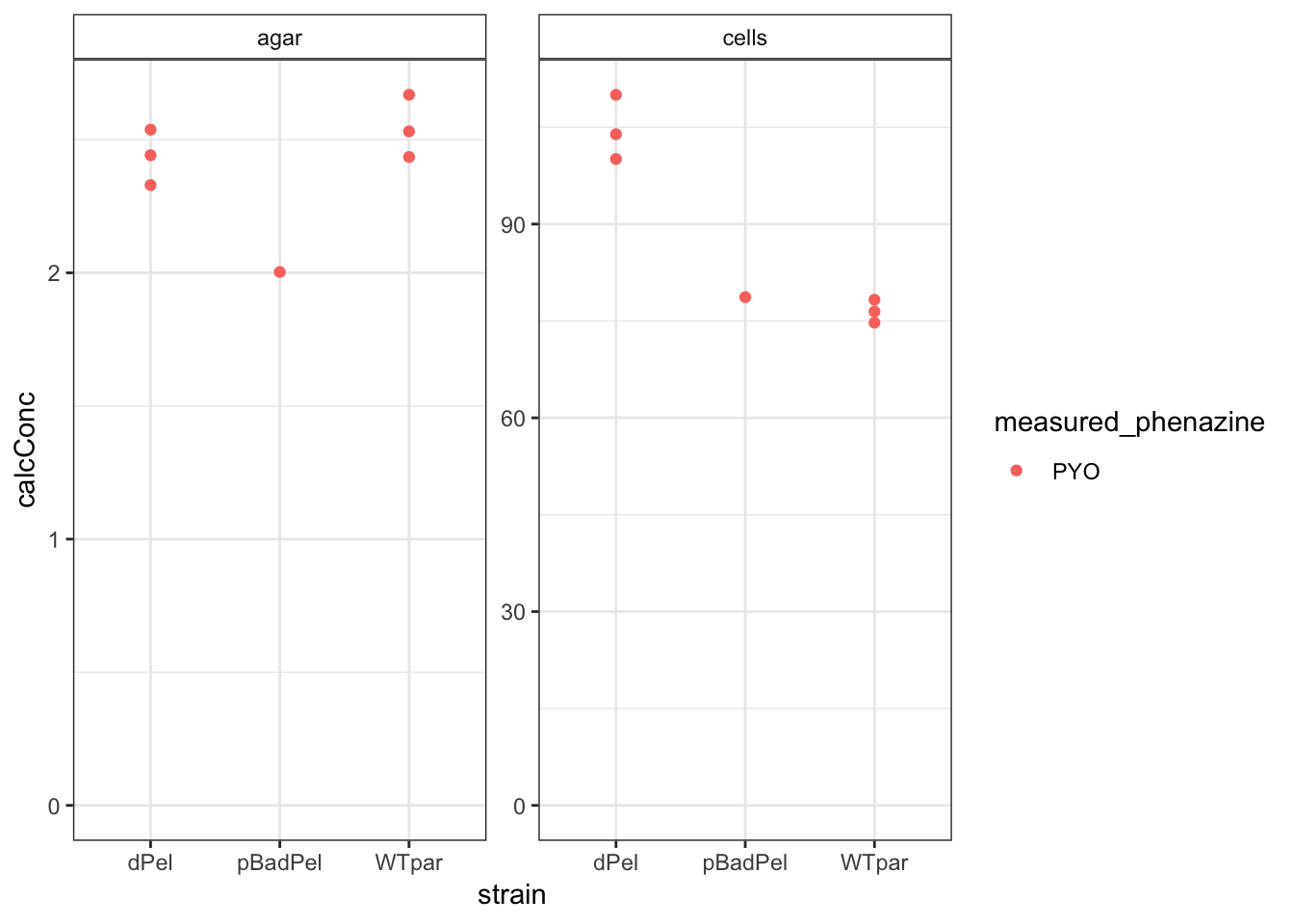

ggplot(df_parsek %>% filter(strain != "pBadPel") %>% filter(material == 
    "cells"), aes(x = strain, y = calcConc, color = measured_phenazine)) + 
    geom_jitter(width = 0.1) + facet_grid(measured_phenazine ~ 
    ., scales = "free") + ylim(0, NA) + theme(strip.background = element_rect(fill = "white"))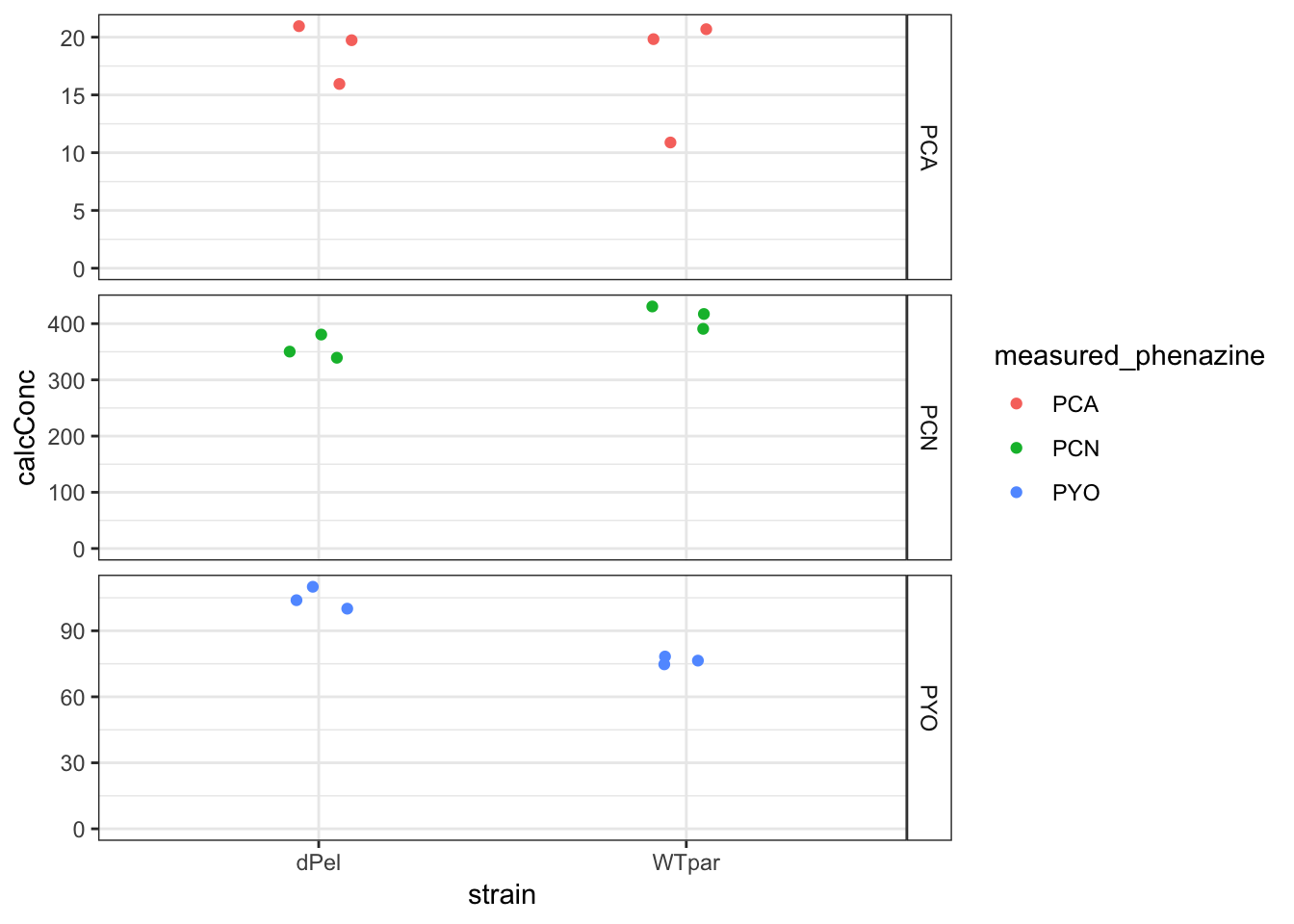

Looks like maybe a real effect for PYO?

df_whit <- df_amounts %>% filter(strain %in% c("WTwhit", "dLys"))

ggplot(df_whit, aes(x = strain, y = calcConc, color = measured_phenazine)) + 
    geom_jitter(width = 0.1) + facet_wrap(measured_phenazine ~ 
    material, scales = "free") + ylim(0, NA) + theme(strip.background = element_rect(fill = "white"))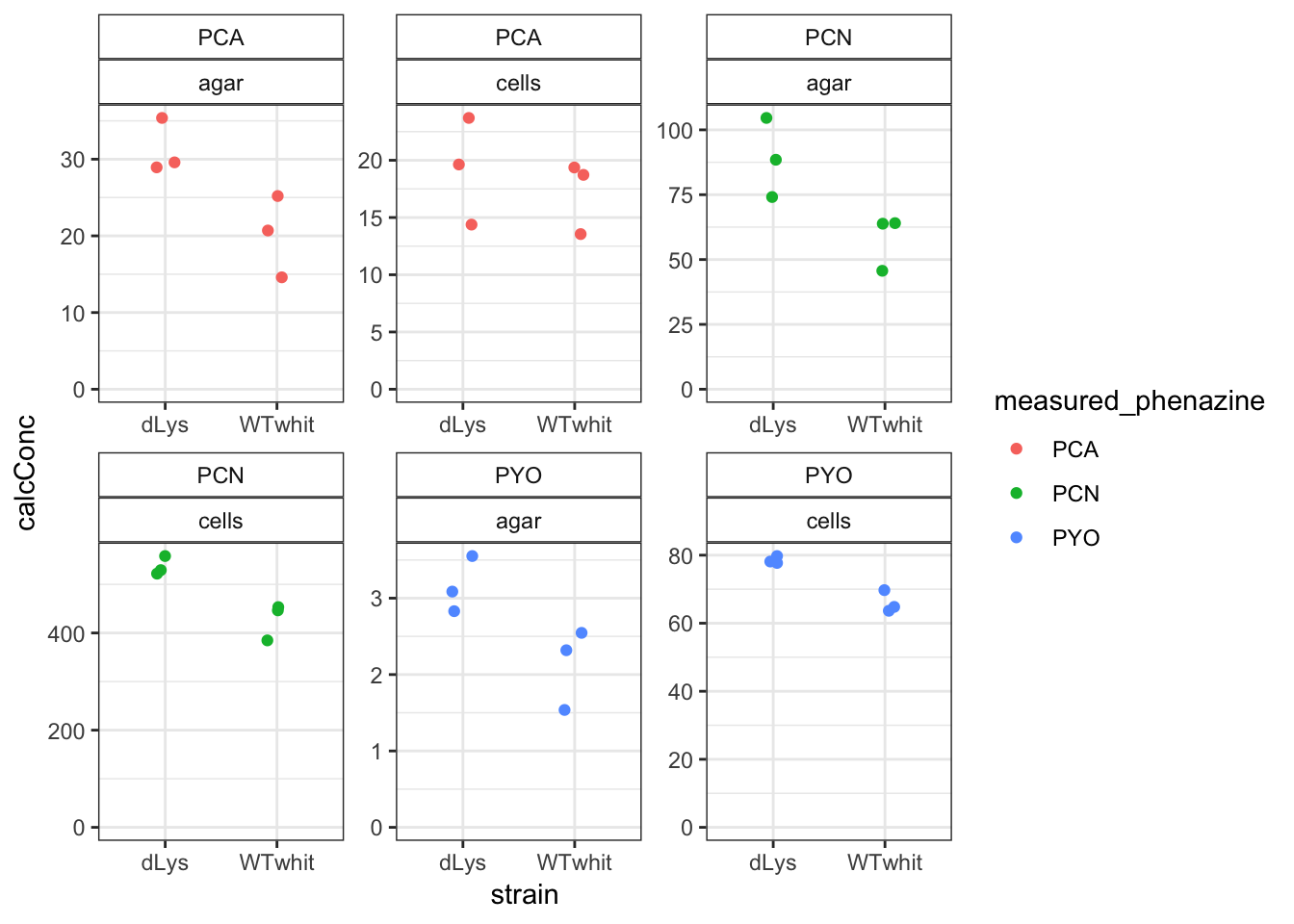

The dLys strain looks like it causes phenazines to reach slightly higher levels in the agar and maybe also in the cells. This is not entirely consistent with the role for eDNA, but it’s worth looking at the actual retention ratios. Also remember that we have no idea how much dLys is contributing to the eDNA in this biofilm - maybe we should measure to be sure.