Measuring \(D_{ap}\) Version 2
Transfer equilibrium titration \(I_{gc}\) vs. [PYO]
1_04_19
library(tidyverse)
library(cowplot)
library(broom)
library(modelr)
library(viridis)
library(lubridate)
library(knitr)

#knitr::opts_knit$set(root.dir = '/Users/scottsaunders/git/labwork/IDA/12_10_18')
knitr::opts_chunk$set(tidy.opts=list(width.cutoff=60),tidy=TRUE, echo = TRUE, message=FALSE, warning=FALSE, fig.align="center")

theme_1 <- function () {
    theme_classic() %+replace%
        theme(
          axis.text = element_text( size=12),
          axis.title=element_text(size=14),
          strip.text = element_text(size = 14),
          strip.background = element_rect(color='white'),
          legend.title=element_text(size=14),
          legend.text=element_text(size=12),
          legend.text.align=0,
          panel.grid.major = element_line(color='grey',size=0.1)
        )
}
theme_set(theme_1())

#source("../../tools/echem_processing_tools.R")
Notebooks that used Version 2 analysis:
- 09_11_18 - Estimating \(D_{ap}\) in triplicate
- 11_28_18 - Estimating \(D_{ap}\) for PYO in solution with blank IDA
Approach
The next approach I took to measuring \(D_{ap}\) was to soak \(\Delta phz\) biofilms with PYO in one reactor and then transfer the biofilms to a second reactor with fresh medium. The echem measurements were then taken in the “transfer” reactor, so that we could be more confident the signal was coming from biofilm associated PYO, not the solution PYO.
In order to do this, I needed a way to estimate the concentration of PYO left in the biofilm when making the measurements. What we settled on is to take a single electrode square wave voltammetry (SWV) scan after taking each generator collector (GC) scan. What we realized was that plotting \(I_{gc}\) vs. \(I_{swv}\) actually yielded a line that depends on \(D_{ap}\), which was what we sought in V1 for the \(I_{gc}\) vs. \(C\) plots.
Derivation for \(D_{ap}\) from \(I_{gc}\) vs. \(I_{swv}\)
\(I_{gc}\) and \(I_{swv}\) depend on \(D_{ap}\) differently, because the currents arise through different processes. \(I_{gc}\) is an equilibrium flux that depends on a diffusion coefficient and concentration gradient similar to fick’s law. \(I_{swv}\) depends on non equilibrium diffusion (fick’s second law) as described by the cottrell equation - while the electrode is poised it constantly changes the concentration gradient.
Slope of the linear fit of GC vs. SWV titration plot: \[slope = m = \frac{\Delta I_{gc}}{\Delta I_{swv}} \tag{eq. 1}\] Generator collector peak current: \[I_{gc} = nFSCD_{ap} \tag{eq. 2}\]
Square Wave peak current: \[I_{swv} = \frac{nFACD_{ap}^{1/2}}{\pi^{1/2}t_p^{1/2}} \psi \tag{eq. 3}\] Substituting into eq. 1: \[m = \frac{I_{gc}}{I_{swv}} = \frac{nFSCD_{ap}}{\frac{nFACD_{ap}^{1/2}}{\pi^{1/2}t_p^{1/2}} \psi} \tag{eq. 4}\] Assuming that \(D_{ap}\) and \(C\) are the same for GC and SWV we can simplify: \[m = \frac{S\pi^{1/2}t_p^{1/2}D_{ap}^{1/2}}{A\psi} \tag{eq. 5}\]
Rearranged for \(D_{ap}\): \[D_{ap} = \frac{m^2 A^2 \psi^2}{S^2\pi t_p} \tag{eq. 7}\]
Therefore, with this dataset in hand, we should be able to estimate \(D_{ap}\) for the biofilm associated PYO, by measuring in the transfer reactor.
Protocol
- Soak biofilm in PYO solution and take GC/SWV.
- Rinse biofilm and transfer to fresh medium reactor.
- Monitor equilibration with successive SWV scans (scan every 2 min).
- At equilibrium take GC scan and final SWV scan.
- Repeat from step 1 with increasing PYO concentrations.
In V1, we were already using a titration approach to vary \(C\), so we continued this approach by soaking the \(\Delta phz\) biofilm in increasing concentrations of synthetic PYO. After each soak, I briefly washed the biofilm and then transferred it to another reactor with fresh medium.
We had reasonably decided to take measurements at a timepoint where the system had reached equilibrium. For various reasons, we assumed that at equilibrium we would only be measuring PYO stably associated with the biofilm, and that the solution concentration was negligible. Two reasons we made these assumptions were that we could transfer the biofilm repeatedly into fresh solution and always detect PYO signal and that measurements on the LC-MS suggested that the solution concentration of PYO was in the nM range, which I thought was below the detection limit of the electrode.
I implemented this protocol by taking successive SWV scans as the biofilm equilibrated in the transfer reactor over the course of ~1 hour. Once the peak SWV current stopped noticeably decreasing, I took a GC and SWV scan. Then I soaked the biofilm in the next higher PYO concentration and repeated for 5-7 concentrations total.
Note that this was quite a long experiment with few datapoints, since each equilibrium datapoint took at least 1.5 hrs and required a potentiostat to monitor the reactor during the entire process.
Problem
In general, V2 titrations looked linear. That said the slope of these \(I_{gc}\) vs. \(I_{swv}\) plots was significantly less for the transfer measurements than measurements taken in the soak reactor (with a biofilm or blank IDA).
gc_swv_equil <- read_csv("../12_04_18_psoralen_biofilm/Processing/12_04_18_processed_gc_swv_equil.csv")

ggplot(gc_swv_equil %>% filter(segment == "1" & condition ==
    "control"), aes(x = signal_from_swv, y = signal_from_gc)) +
    geom_point() + geom_line()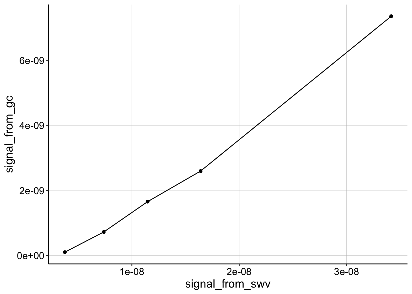
After doing these experiments for a while thinking things were fine, I finally decided to explicitly measure background signal in the transfer reactor (Lenny had suggested this long ago). Below is a plot of the transfer reactor measured “at equilibrium” after an hour with a biofilm coated IDA, followed by a blank IDA.
blank_GC_scans <- read_csv("../12_04_18_psoralen_biofilm/Processing/12_04_18_processed_blank_GC_scans.csv")

ggplot(blank_GC_scans %>% filter(E < 0 & condition == "control"),
    aes(x = E, y = current, color = blank)) + geom_path(size = 1) +
    facet_wrap(~PHZadded, scales = "free") + ylim(0, 1.5e-08) +
    scale_x_reverse()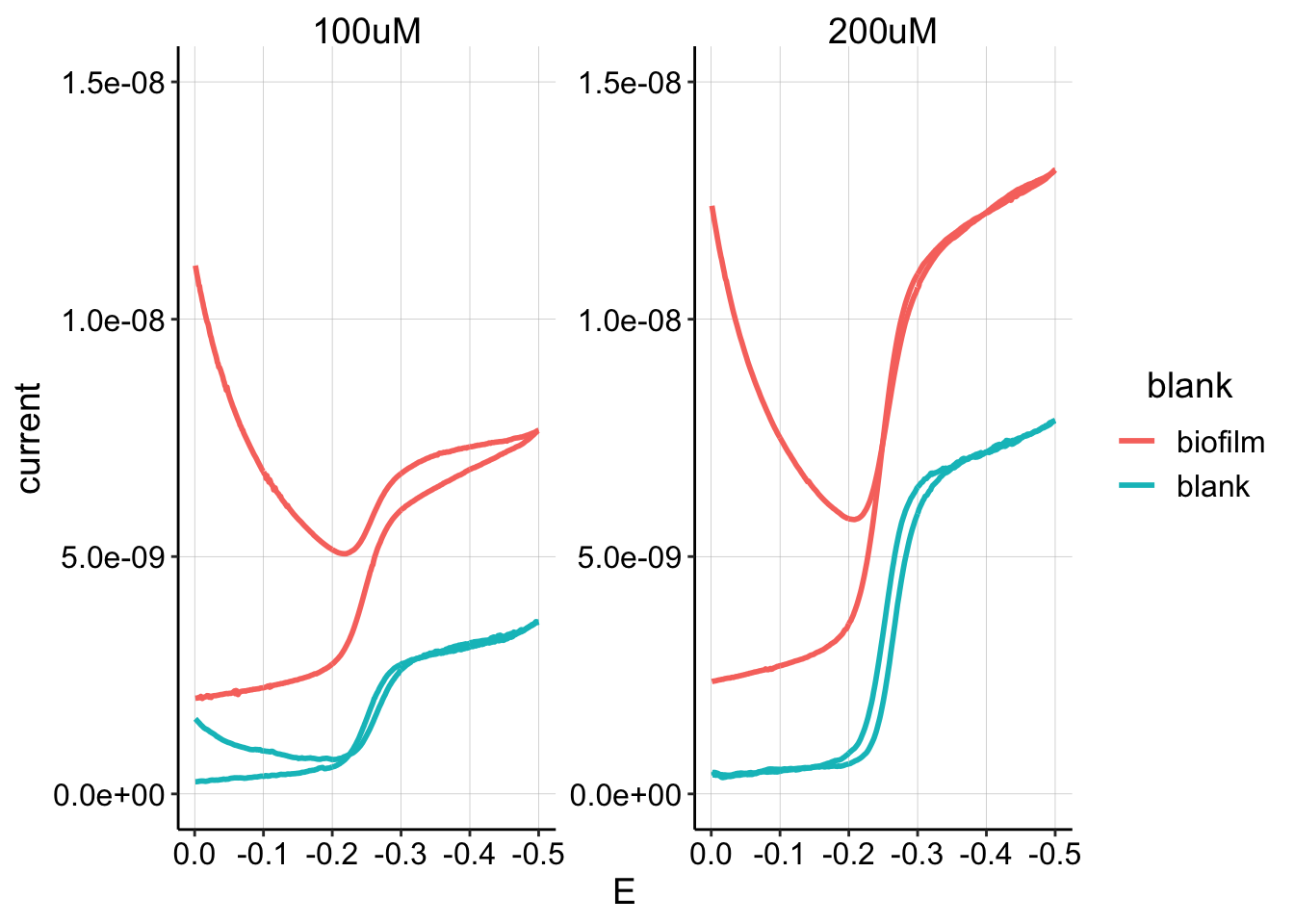
It is clear that the amount of background signal from PYO in solution is significant in these measurements. It is unclear if all of the observed biofilm signal is due to the solution or not. One approach might be to try to background subtract the signal from the blank electrode from the biofilm electrode, however, this assumes \(I_{gc} = I_{biofilm} + I_{blank}\). We know that this is not true in the soak phase, because the biofilm electrode actually shows less signal than the blank electrode. Therefore any attempt to background subtract would get impractically complicated (you probably need to know fraction of electrode exposed to solution, \(D_{ap}\) for each phase, and concentrations).
Conclusions
Good
- The derivation for \(D_{ap}\) from \(I_{gc}\) vs. \(I_{swv}\) is still valid. It produces a reasonable value for \(D_{ap}\) of solution PYO at a blank IDA.
- The process of using SWV to monitor the PYO equilibration out of the biofilm led to the idea of measuring \(D_m\).
Bad
- The electrode was more sensitive than I realized, and therefore the background signal from the PYO in solution was much higher than I expected.
Solutions
- Make GC/SWV measurements during equilibration, before solution/background is relatively significant.
- Reduce PYO carryover by soaking only IDA working surface
- Explicitly measure background in transfer reactor with blank IDA.