library(tidyverse)
library(cowplot)
library(broom) 
library(modelr) 
library(viridis)
library(lubridate)
library(hms)
library(knitr)
library(kableExtra)

knitr::opts_chunk$set(tidy.opts=list(width.cutoff=60),tidy=TRUE, echo = TRUE, message=FALSE, warning=FALSE, fig.align="center")

source("../../tools/echem_processing_tools.R")
source("../../tools/plotting_tools.R")

theme_set(theme_1())

soak_1_path = "../data/soak_1/"

tran_1_path = "../data/transfer_1/"

data_cols <- c("E", "i1", "i2")

swv_skip_rows = 18

gc_skip_rows = 21

All SWVs

# Add 'reactor' to file name so it is parsed into column
filename_cols = c("reactor", "echem", "rep")

swv_tran_1_names <- dir(path = tran_1_path, pattern = "[swv]+.+[txt]$") %>% 
    paste("tran1", ., sep = "_")
swv_soak_1_names <- dir(path = soak_1_path, pattern = "[swv]+.+[txt]$") %>% 
    paste("soak1", ., sep = "_")

# Add correct paths separate from filenames
swv_tran_1_paths <- dir(path = tran_1_path, pattern = "[swv]+.+[txt]$") %>% 
    paste(tran_1_path, ., sep = "")
swv_soak_1_paths <- dir(path = soak_1_path, pattern = "[swv]+.+[txt]$") %>% 
    paste(soak_1_path, ., sep = "")

# Combine all SWVs into single vector
swv_names <- c(swv_tran_1_names, swv_soak_1_names)
swv_paths <- c(swv_tran_1_paths, swv_soak_1_paths)

# Read in all SWVs with one function call
swv_data <- echem_import_to_df(filenames = swv_names, file_paths = swv_paths, 
    data_cols = data_cols, skip_rows = swv_skip_rows, filename_cols = filename_cols, 
    rep = T, PHZadded = F)

swv_data %>% head() %>% kable() %>% kable_styling()

reactor	echem	rep	minutes	E	electrode	current
tran1	swv	1	1334.583	0.099	i1	2.1e-06
tran1	swv	1	1334.583	0.098	i1	3.1e-06
tran1	swv	1	1334.583	0.097	i1	3.1e-06
tran1	swv	1	1334.583	0.096	i1	3.1e-06
tran1	swv	1	1334.583	0.095	i1	3.1e-06
tran1	swv	1	1334.583	0.094	i1	3.1e-06

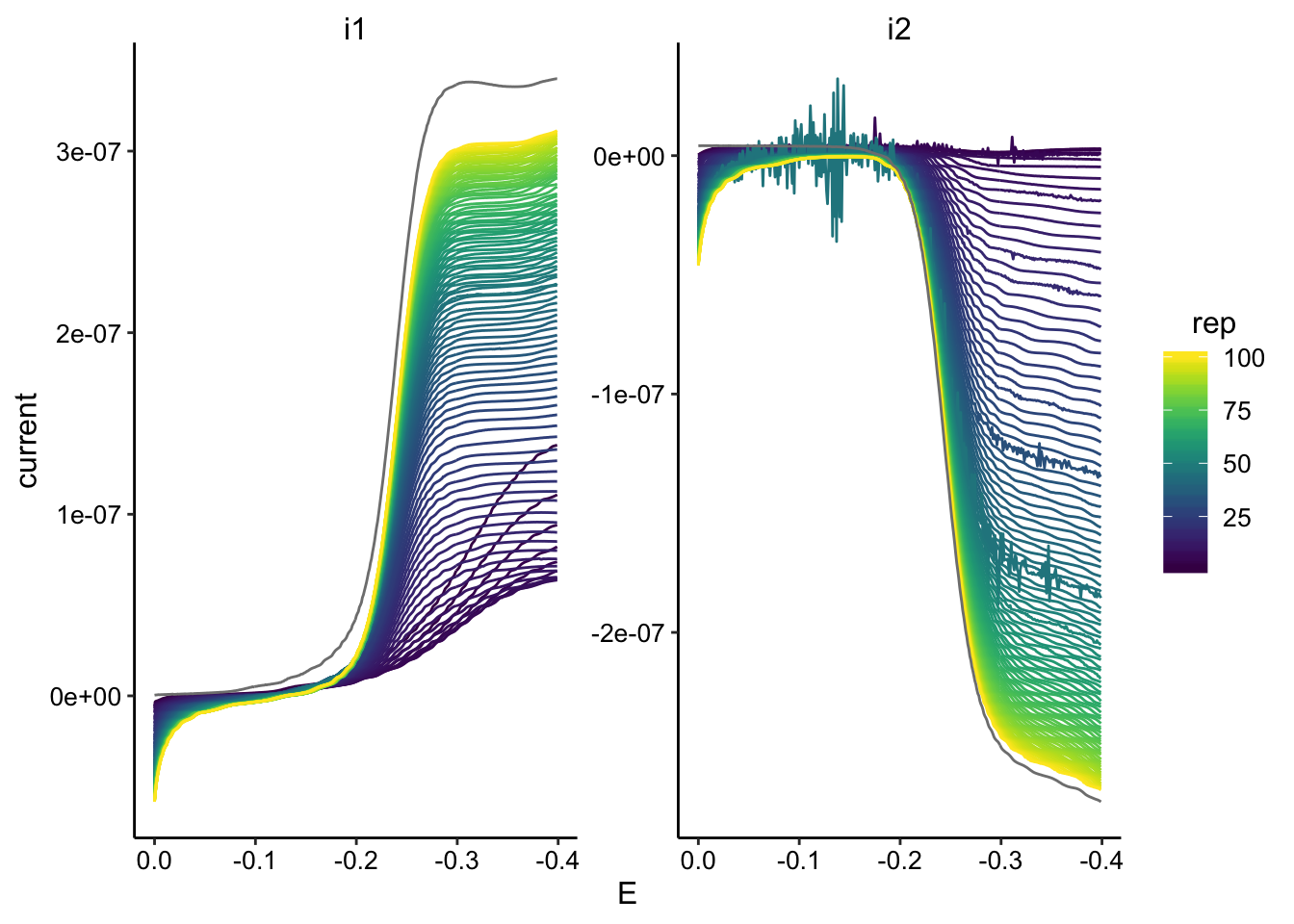
swv_data %>% filter(reactor == "soak1") %>% ggplot(., aes(x = E, 
    y = current, color = rep, group = rep)) + geom_path() + facet_wrap(~electrode, 
    scales = "free") + scale_color_viridis() + scale_x_reverse()

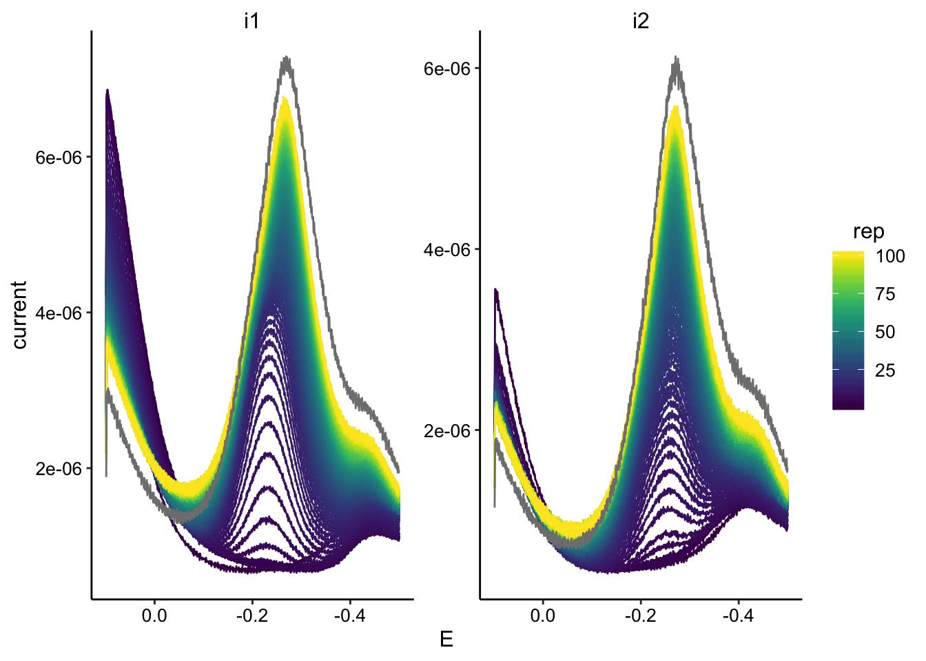
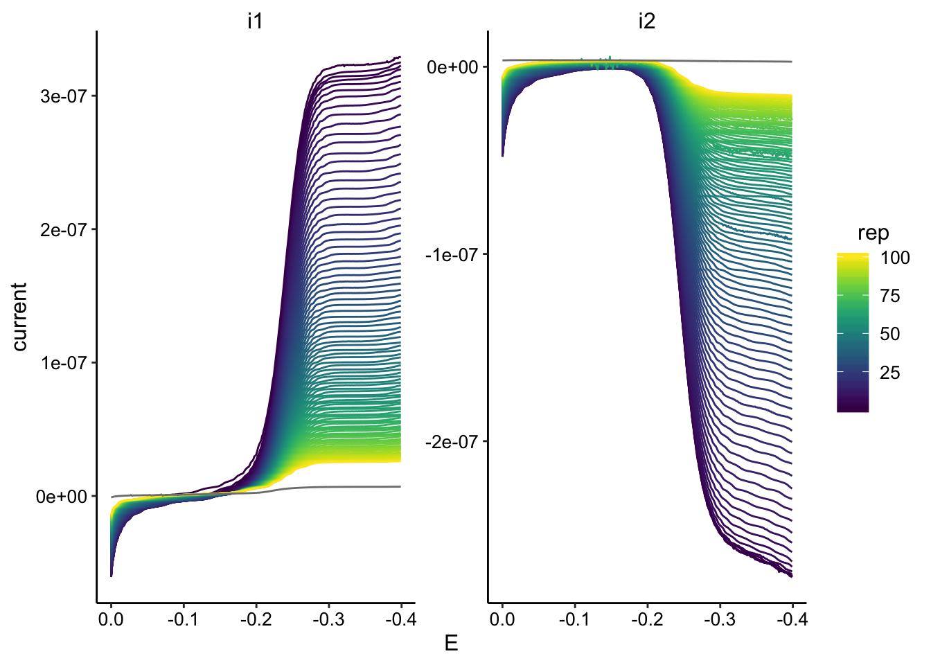
swv_data %>% filter(reactor == "tran1") %>% ggplot(., aes(x = E, 
    y = current, color = rep, group = rep)) + geom_path() + facet_wrap(~electrode, 
    scales = "free") + scale_color_viridis() + scale_x_reverse()

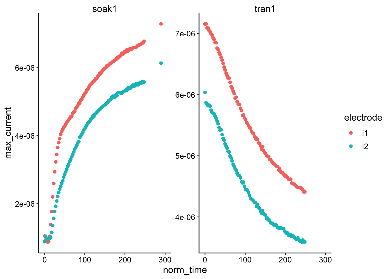
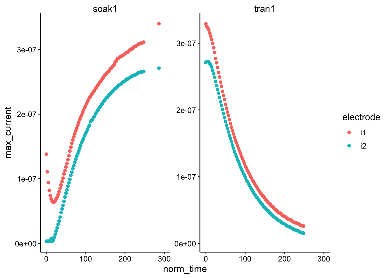
swv_max <- swv_data %>% mutate(minutes = ifelse(minutes < 1000, 
    minutes + 1440, minutes)) %>% 
group_by(reactor) %>% mutate(min_time = min(minutes)) %>% mutate(norm_time = minutes - 
    min_time) %>% 
group_by(reactor, rep, electrode) %>% filter(E < -0.15 & E > 
    -0.35) %>% mutate(max_current = max(abs(current))) %>% filter(abs(current) == 
    max_current)

ggplot(swv_max, aes(x = norm_time, y = max_current, color = electrode)) + 
    geom_point() + facet_wrap(~reactor, scales = "free") + xlim(0, 
    300)

All GCs

# Add 'reactor' to file name so it is parsed into column
filename_cols = c("reactor", "echem", "rep")

gc_tran_1_names <- dir(path = tran_1_path, pattern = "[gc]+.+[txt]$") %>% 
    paste("tran1", ., sep = "_")
gc_soak_1_names <- dir(path = soak_1_path, pattern = "[gc]+.+[txt]$") %>% 
    paste("soak1", ., sep = "_")

# Add correct paths separate from filenames
gc_tran_1_paths <- dir(path = tran_1_path, pattern = "[gc]+.+[txt]$") %>% 
    paste(tran_1_path, ., sep = "")
gc_soak_1_paths <- dir(path = soak_1_path, pattern = "[gc]+.+[txt]$") %>% 
    paste(soak_1_path, ., sep = "")

# Combine all SWVs into single vector
gc_names <- c(gc_tran_1_names, gc_soak_1_names)
gc_paths <- c(gc_tran_1_paths, gc_soak_1_paths)

# Read in all SWVs with one function call
gc_data <- echem_import_to_df(filenames = gc_names, file_paths = gc_paths, 
    data_cols = data_cols, skip_rows = gc_skip_rows, filename_cols = filename_cols, 
    rep = T, PHZadded = F)

gc_data %>% head() %>% kable(digits = 9) %>% kable_styling()

reactor	echem	rep	minutes	E	electrode	current
tran1	gc	1	1336.9	0.000	i1	-4.1e-08
tran1	gc	1	1336.9	-0.001	i1	-3.5e-08
tran1	gc	1	1336.9	-0.002	i1	-3.3e-08
tran1	gc	1	1336.9	-0.003	i1	-2.8e-08
tran1	gc	1	1336.9	-0.004	i1	-2.7e-08
tran1	gc	1	1336.9	-0.005	i1	-2.3e-08

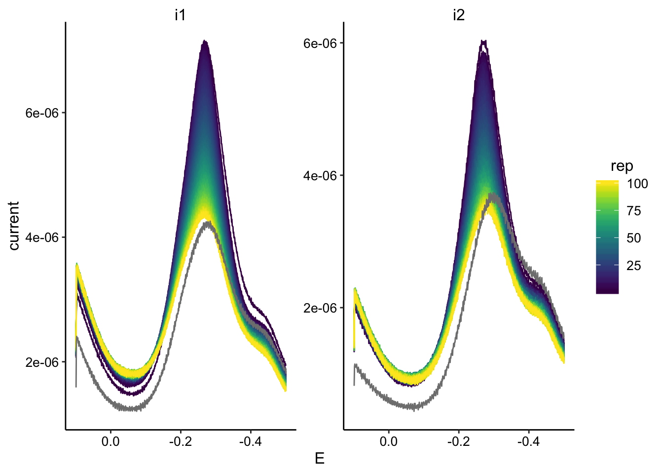
gc_data %>% filter(reactor == "soak1") %>% ggplot(., aes(x = E, 
    y = current, color = rep, group = rep)) + geom_path() + facet_wrap(~electrode, 
    scales = "free") + scale_color_viridis() + scale_x_reverse()

gc_data %>% filter(reactor == "tran1") %>% ggplot(., aes(x = E, 
    y = current, color = rep, group = rep)) + geom_path() + facet_wrap(~electrode, 
    scales = "free") + scale_color_viridis() + scale_x_reverse()

gc_max <- gc_data %>% mutate(minutes = ifelse(minutes < 1000, 
    minutes + 1440, minutes)) %>% 
group_by(reactor) %>% mutate(min_time = min(minutes)) %>% mutate(norm_time = minutes - 
    min_time) %>% 
group_by(reactor, rep, electrode) %>% filter(E < -0.2) %>% mutate(max_current = max(abs(current))) %>% 
    filter(abs(current) == max_current)

ggplot(gc_max, aes(x = norm_time, y = max_current, color = electrode)) + 
    geom_point() + facet_wrap(~reactor, scales = "free") + xlim(0, 
    300)

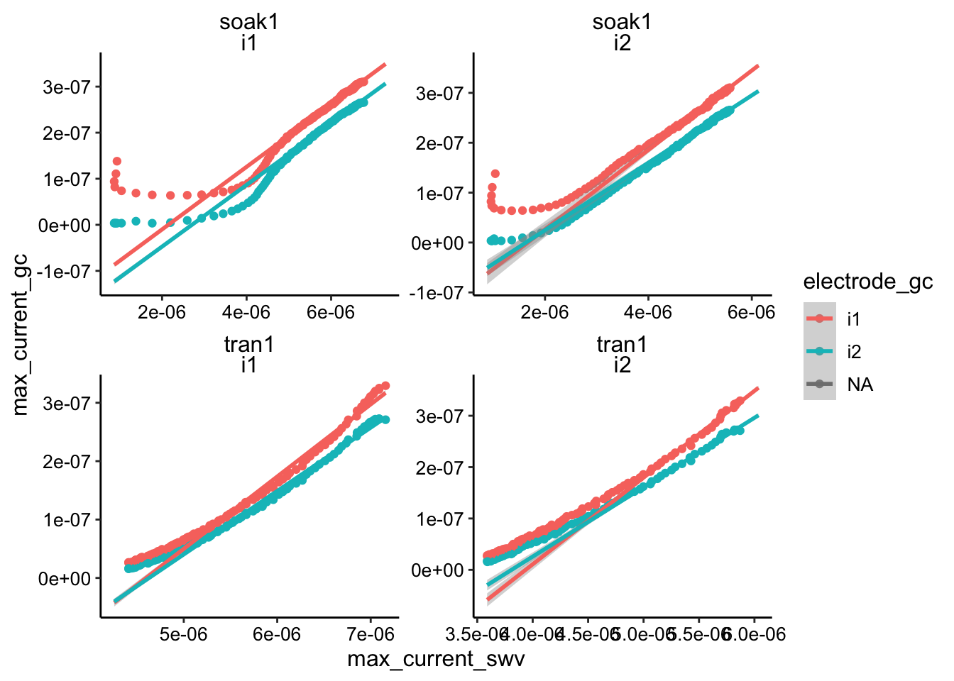
SWV vs. GC

swv_gc_max <- left_join(swv_max %>% ungroup() %>% mutate(rep = rep - 
    1), gc_max, by = c("reactor", "rep"), suffix = c("_swv", 
    "_gc"))

ggplot(swv_gc_max, aes(x = max_current_swv, y = max_current_gc, 
    color = electrode_gc)) + geom_point() + geom_smooth(data = swv_gc_max %>% 
    filter(max_current_swv > 5e-06), method = "lm", fullrange = T) + 
    facet_wrap(c("reactor", "electrode_swv"), scales = "free")

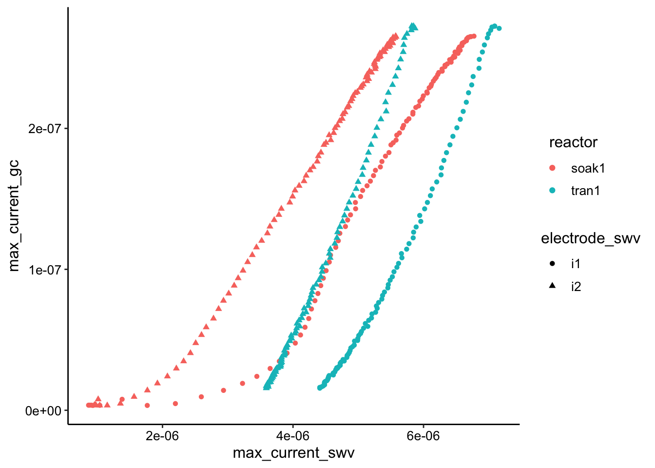
ggplot(swv_gc_max %>% filter(electrode_gc == "i2"), aes(x = max_current_swv, 
    y = max_current_gc, color = reactor, shape = electrode_swv)) + 
    geom_point()

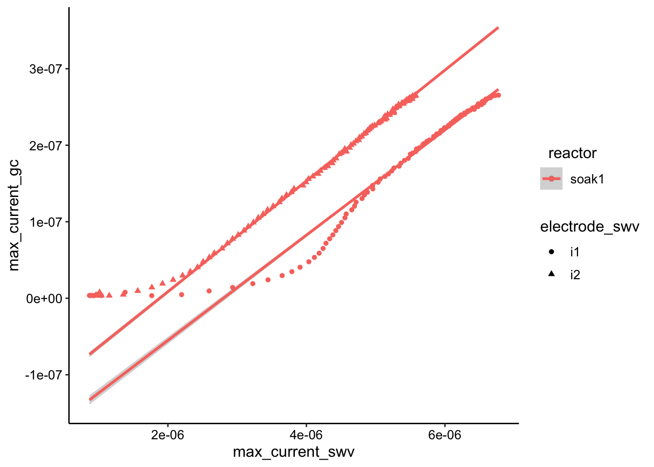
ggplot(swv_gc_max %>% filter(electrode_gc == "i2" & reactor == 
    "soak1"), aes(x = max_current_swv, y = max_current_gc, color = reactor, 
    shape = electrode_swv)) + geom_point() + geom_smooth(data = swv_gc_max %>% 
    filter(electrode_gc == "i2" & reactor == "soak1" & rep > 
        30), method = "lm", fullrange = T)

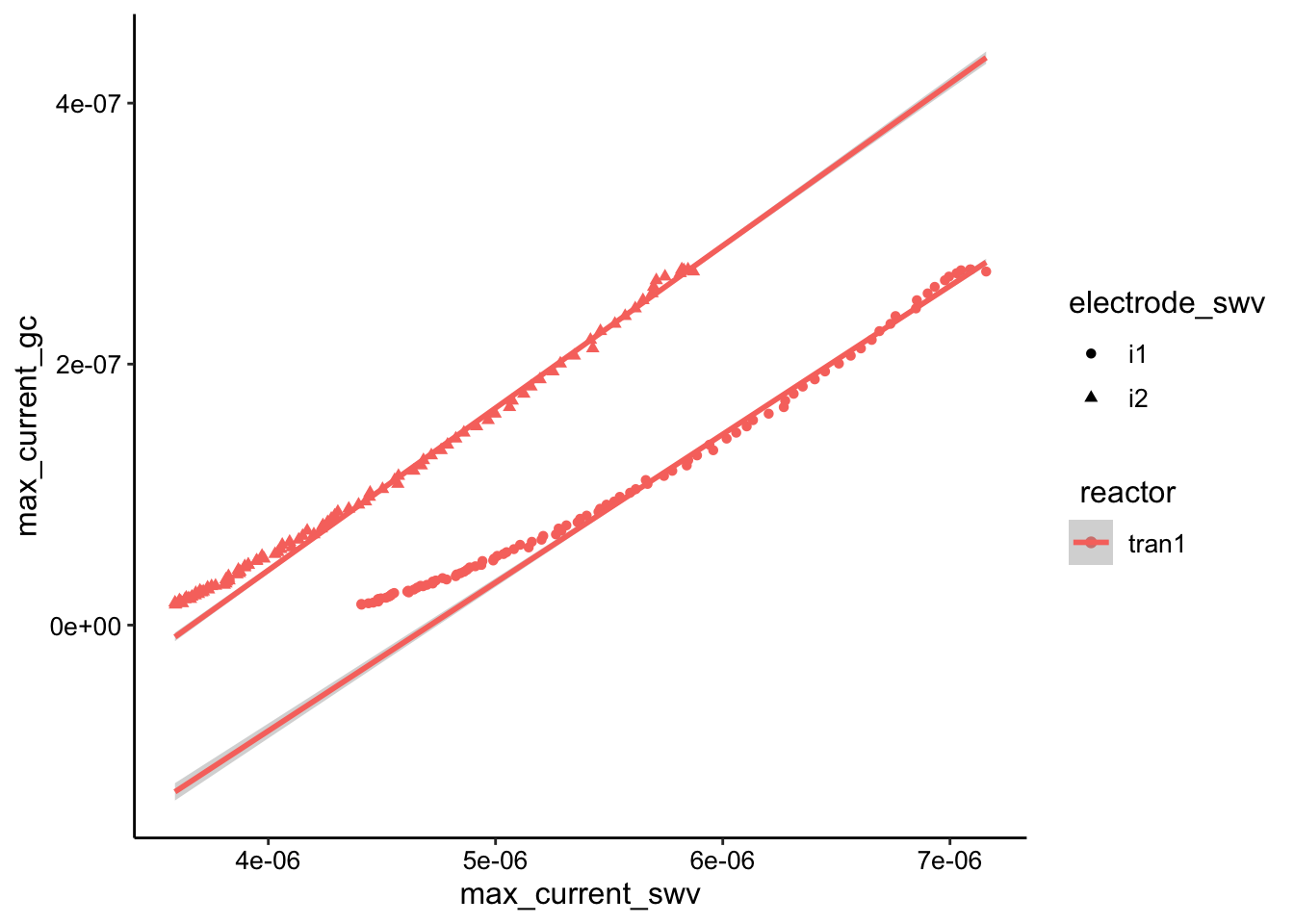
ggplot(swv_gc_max %>% filter(electrode_gc == "i2" & reactor == 
    "tran1"), aes(x = max_current_swv, y = max_current_gc, color = reactor, 
    shape = electrode_swv)) + geom_point() + geom_smooth(data = swv_gc_max %>% 
    filter(electrode_gc == "i2" & reactor == "tran1" & rep < 
        50), method = "lm", fullrange = T)

dap_from_swvGC <- function(m, t_p = 1/(2 * 300)) {
    
    psi <- 0.7
    # psi <- 0.75 A <- 0.013 #cm^2
    A <- 0.025  #cm^2
    S <- 18.4  #cm
    d_ap <- (m * A * psi)^2/(S^2 * pi * t_p)
    
    d_ap
}

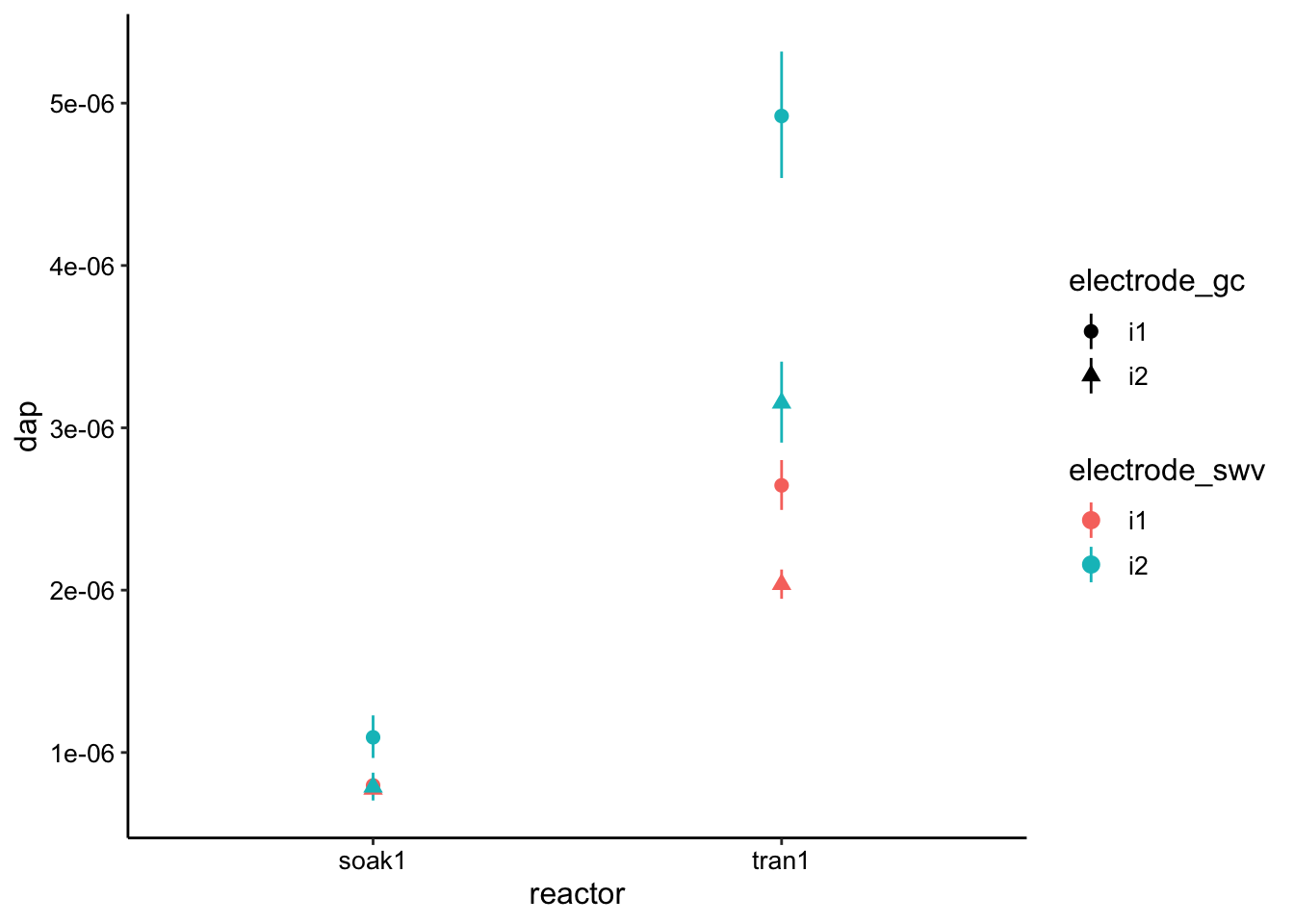
lms <- swv_gc_max %>% filter(rep > 0 & max_current_swv > 5e-06) %>% 
    group_by(reactor, electrode_swv, electrode_gc) %>% do(tidy(lm(max_current_gc ~ 
    max_current_swv, data = .), conf.int = T)) %>% filter(term == 
    "max_current_swv") %>% mutate(dap = dap_from_swvGC(m = estimate)) %>% 
    mutate(dap_high = dap_from_swvGC(m = conf.high)) %>% mutate(dap_low = dap_from_swvGC(m = conf.low)) %>% 
    mutate(dataset = "SWVvsGC")

lms %>% kable() %>% kable_styling()

reactor	electrode_swv	electrode_gc	term	estimate	std.error	statistic	conf.low	conf.high	dap	dap_high	dap_low	dataset
soak1	i1	i1	max_current_swv	0.0679339	0.0003857	176.11233	0.0671629	0.0687050	8.0e-07	8.0e-07	8.0e-07	SWVvsGC
soak1	i1	i2	max_current_swv	0.0669625	0.0005771	116.02347	0.0658088	0.0681162	8.0e-07	8.0e-07	7.0e-07	SWVvsGC
soak1	i2	i1	max_current_swv	0.0795563	0.0023490	33.86869	0.0747826	0.0843300	1.1e-06	1.2e-06	1.0e-06	SWVvsGC
soak1	i2	i2	max_current_swv	0.0675213	0.0018069	37.36832	0.0638493	0.0711934	8.0e-07	9.0e-07	7.0e-07	SWVvsGC
tran1	i1	i1	max_current_swv	0.1237482	0.0017951	68.93727	0.1201563	0.1273402	2.6e-06	2.8e-06	2.5e-06	SWVvsGC
tran1	i1	i2	max_current_swv	0.1085590	0.0012016	90.34606	0.1061546	0.1109634	2.0e-06	2.1e-06	1.9e-06	SWVvsGC
tran1	i2	i1	max_current_swv	0.1687697	0.0032219	52.38178	0.1620878	0.1754515	4.9e-06	5.3e-06	4.5e-06	SWVvsGC
tran1	i2	i2	max_current_swv	0.1351031	0.0025761	52.44495	0.1297606	0.1404456	3.2e-06	3.4e-06	2.9e-06	SWVvsGC

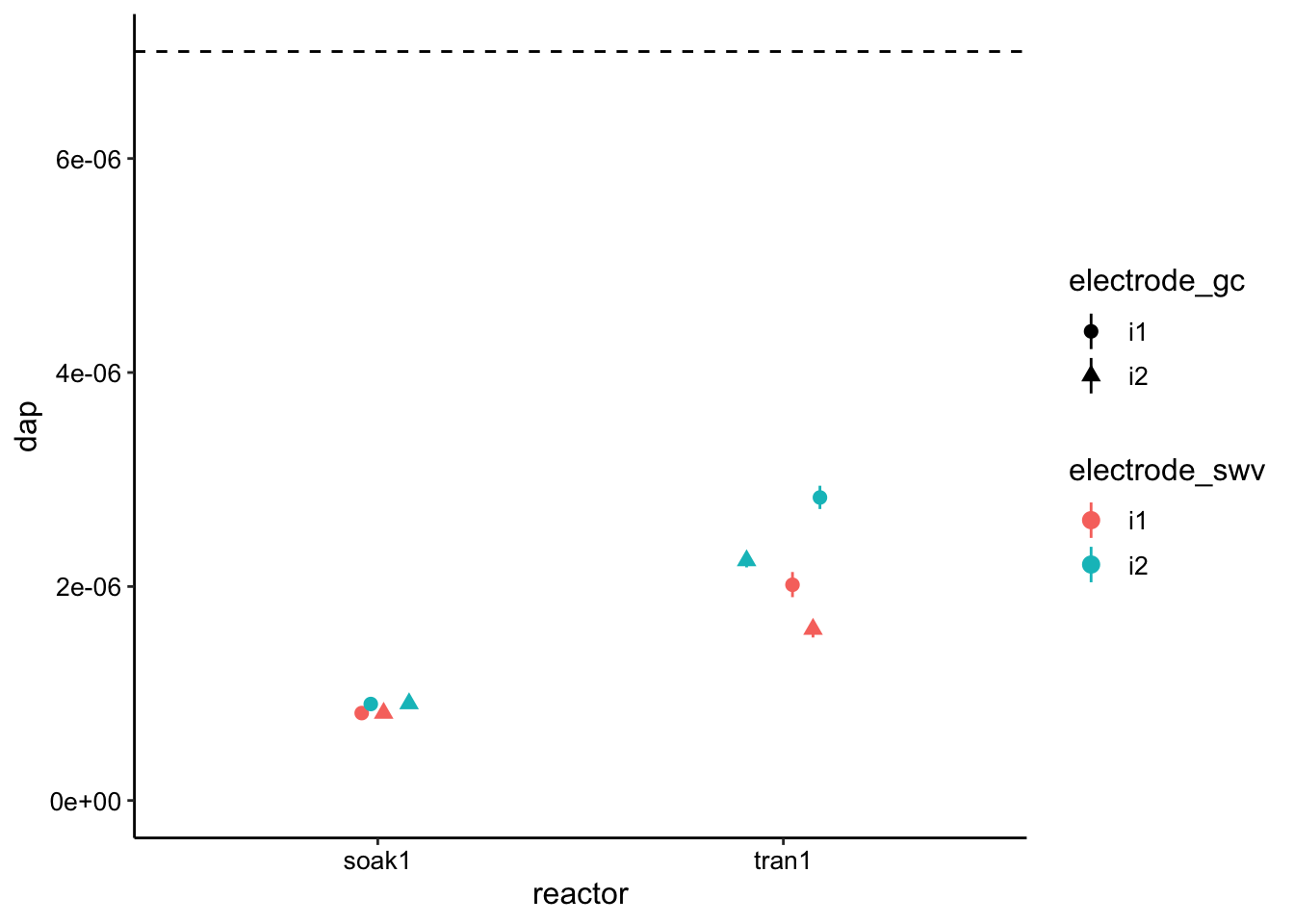
ggplot(lms, aes(x = reactor, y = dap, color = electrode_swv, 
    shape = electrode_gc)) + geom_pointrange(aes(ymin = dap_low, 
    ymax = dap_high))

lm_soak <- swv_gc_max %>% filter(reactor == "soak1") %>% filter(rep > 
    0 & rep > 30) %>% group_by(reactor, electrode_swv, electrode_gc) %>% 
    do(tidy(lm(max_current_gc ~ max_current_swv, data = .), conf.int = T)) %>% 
    filter(term == "max_current_swv") %>% mutate(dap = dap_from_swvGC(m = estimate)) %>% 
    mutate(dap_high = dap_from_swvGC(m = conf.high)) %>% mutate(dap_low = dap_from_swvGC(m = conf.low)) %>% 
    mutate(dataset = "SWVvsGC")

lm_tran <- swv_gc_max %>% filter(reactor == "tran1") %>% filter(rep > 
    0 & max_current_swv < 50) %>% group_by(reactor, electrode_swv, 
    electrode_gc) %>% do(tidy(lm(max_current_gc ~ max_current_swv, 
    data = .), conf.int = T)) %>% filter(term == "max_current_swv") %>% 
    mutate(dap = dap_from_swvGC(m = estimate)) %>% mutate(dap_high = dap_from_swvGC(m = conf.high)) %>% 
    mutate(dap_low = dap_from_swvGC(m = conf.low)) %>% mutate(dataset = "SWVvsGC")

bind_rows(lm_soak, lm_tran) %>% ggplot(., aes(x = reactor, y = dap, 
    color = electrode_swv, shape = electrode_gc)) + geom_hline(yintercept = 7e-06, 
    linetype = 2) + geom_pointrange(aes(ymin = dap_low, ymax = dap_high), 
    position = position_jitter(width = 0.1, height = 0)) + ylim(0, 
    NA)

Agarose Glycerol

Processing

Scott Saunders

08_15_19

All SWVs

All GCs

SWV vs. GC