Analysis

Estimating \(D_{ap}\) from GC/SWV

Let’s just plot all of the SWV signals vs. the GC signals. As we move forward, there may be reasons to use one subset of the data over others, but let’s start here.

ggplot(gc_swv_df, aes(x = signal_from_swv, y = signal_from_gc, 
    color = PHZadded)) + geom_point()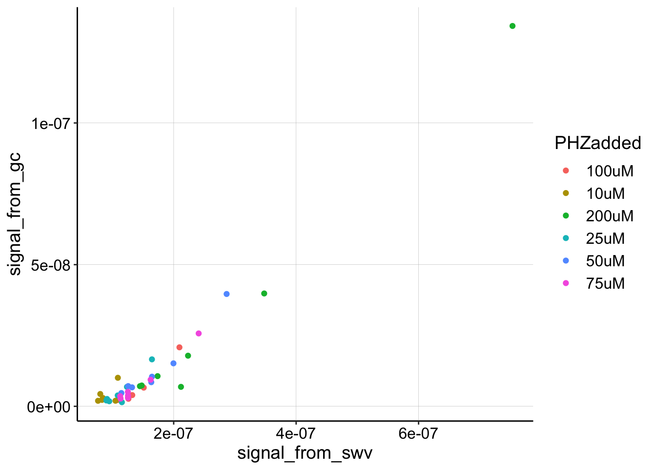

This plot actually looks pretty linear, so across the different concentrations we soaked the biofilm in we might have actually gotten a pretty consistent measurement.

The 200uM data points make it a little harder to look at the rest of the data, so let’s ignore them for a different look.

ggplot(gc_swv_df %>% filter(PHZaddedInt < 200), aes(x = signal_from_swv, 
    y = signal_from_gc, color = PHZadded)) + geom_point()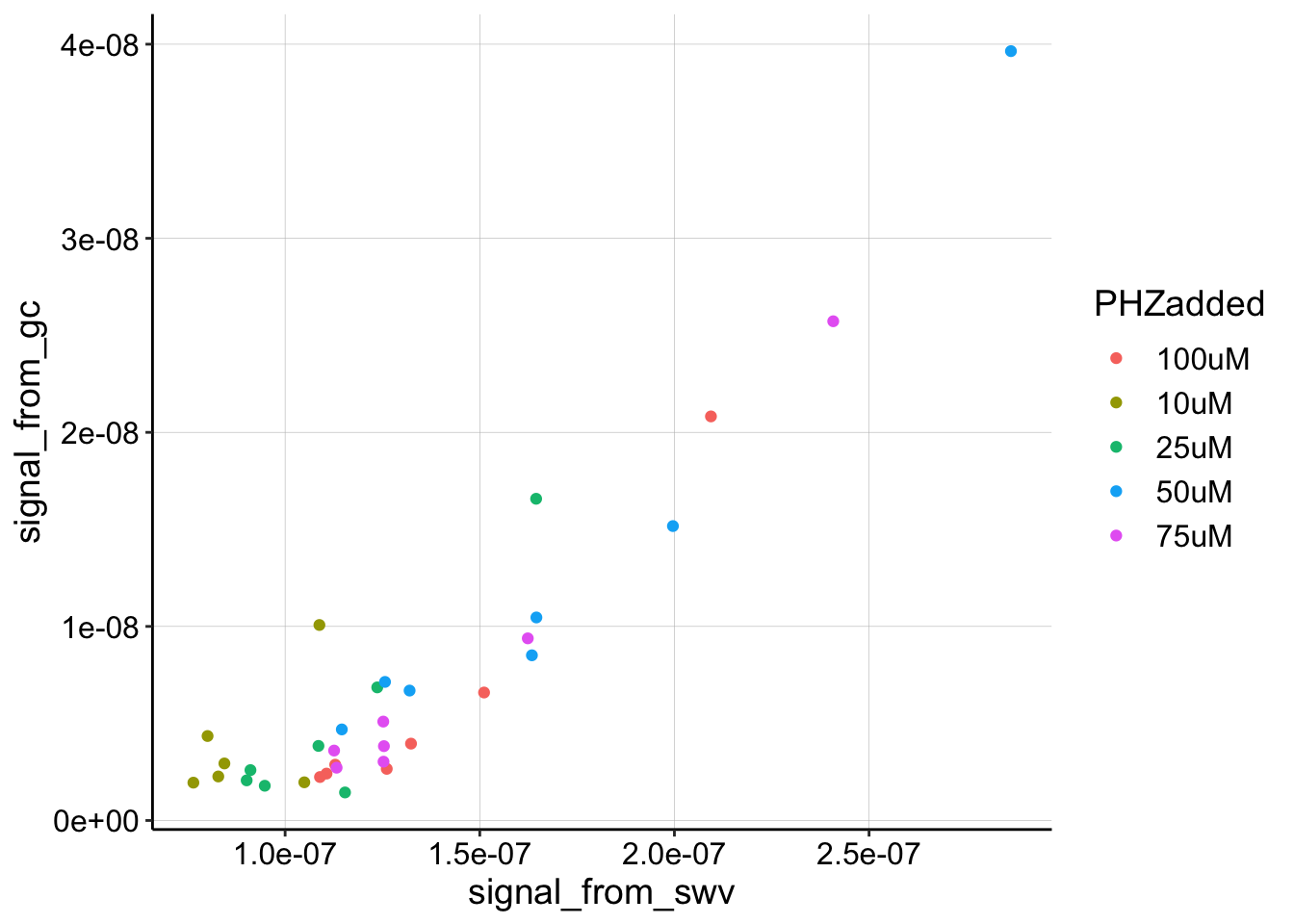

Ok, this plot still looks reasonably consistent. There still seems to be a strong linear increase in GC signal as SWV signal increases. There’s likely some noise in how we quantified the data at the lowest signals, especially for the 10uM level. I think that we could go back to the data and try to loess smooth to get more accurate quantification, but for now, let’s also ignore the 10uM level and fit a linear model to see how it looks.

ggplot(gc_swv_df %>% filter(PHZaddedInt < 200 & PHZaddedInt > 
    10), aes(x = signal_from_swv, y = signal_from_gc)) + geom_point(aes(color = PHZadded)) + 
    geom_smooth(method = "lm")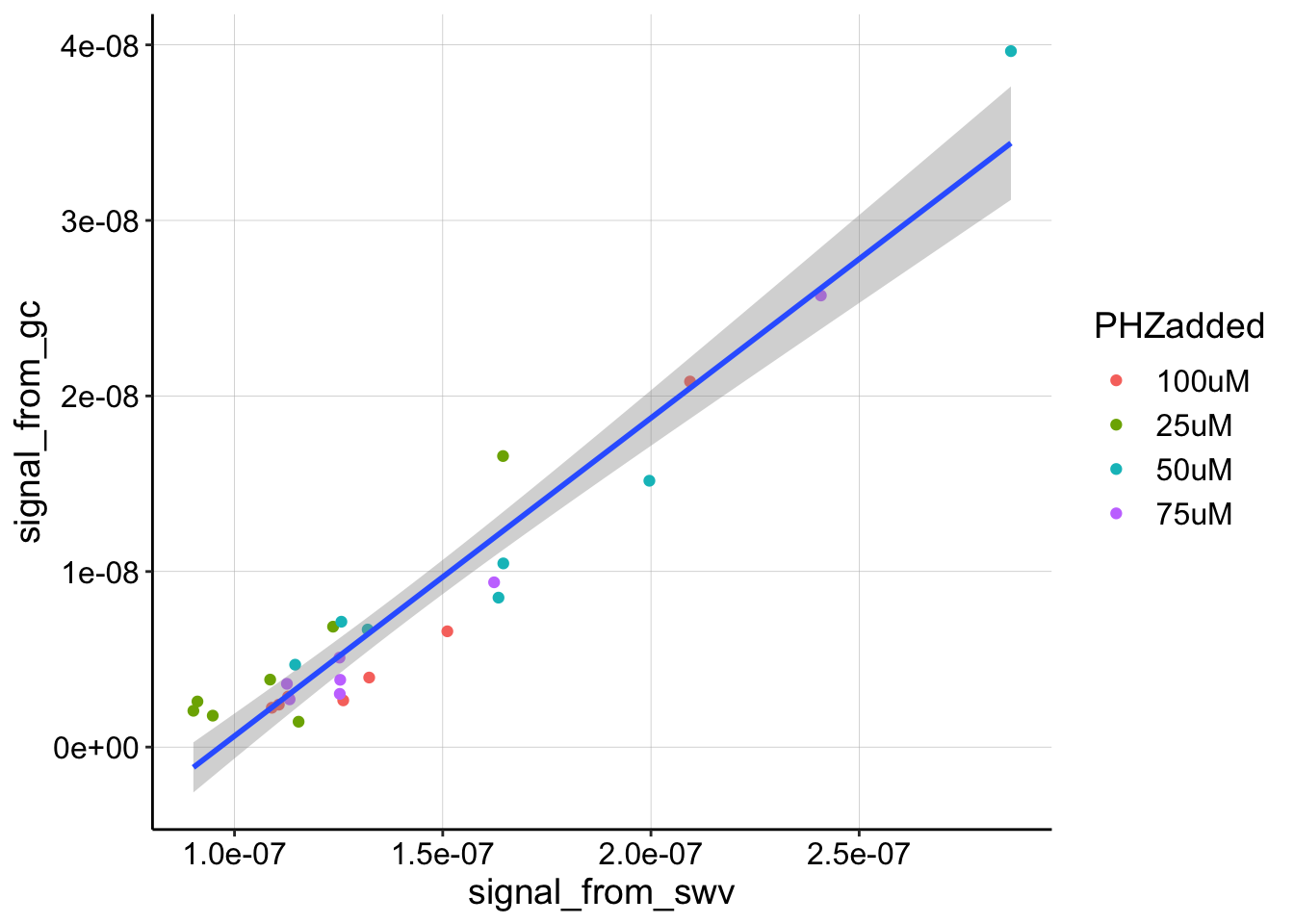

Again, the linear fit isn’t perfect, but it seems like a reasonable approximation. Let’s grab the slope coefficient from the linear fit, so that we can estimate a \(D_{ap}\)

gc_swv_linear_fit1 <- lm(signal_from_gc ~ signal_from_swv, gc_swv_df %>% 
    filter(PHZaddedInt < 200 & PHZaddedInt > 10))

coef(summary(gc_swv_linear_fit1))

##                      Estimate  Std. Error   t value     Pr(>|t|)
## (Intercept)     -1.748189e-08 1.51598e-09 -11.53174 1.007475e-11
## signal_from_swv  1.811346e-01 1.02817e-02  17.61718 5.656763e-16

So this linear fit is telling us that the slope, \(m\) of the best fit line is about 0.18 +/- 0.01. That’s a pretty confident estimate, and the small p value is telling us that the slope is definitely not zero.

Recall that \(D_{ap}\) is

\[ D_{ap} = \frac{(m A \psi)^2 }{S^2 \pi t_p }\]

Therefore, for this data with the following parameters yields the following \(D_{ap}\):

m <- 0.18

psi <- 0.91
t_p <- 1/300  # frequency is 300 hz (sec)
A <- 0.025  #cm^2
S <- 18.4  #cm
D_ap <- (m * A * psi)^2/(S^2 * pi * t_p)

paste("D_ap =", D_ap, "cm^2 / sec")

## [1] "D_ap = 4.72980839954201e-06 cm^2 / sec"

So the estimate from this data is that \(D_{ap}\) is around 4.7 x 10^-6 cm^2 / sec, which is similar to the estimates we obtained before!

We could estimate this parameter individually for each level of the titration, but the points look like they will have pretty similar slopes. However, note that small variations in m affect Dap in a nonlinear (squared) manner. For example m=0.1 yields D_ap=1.5e-6. That said, I think the point stands, that we expect D_ap to fall within this order of magnitude.

Estimating \(D_m\) from SWV decays

Let’s read in the data from the SWVs from all the titration points. Remember, 5 swvs were taken, then a GC then 5 more swvs etc.

swv_decays <- read_csv("../Processing/12_10_18_processed_reactor_A_swv_decays.csv")

In order to fit the nonlinear decay to these plots let’s normalize to the highest signal, and consider it as the initial signal.

swv_decays_norm <- swv_decays %>% group_by(PHZadded) %>% mutate(I0 = max(signal)) %>% 
    mutate(norm_signal = signal/I0)

Now we can fit the remaining datapoints (just not the first one).

ggplot(swv_decays_norm %>% filter(rep != 0 | sub_rep != 1), aes(x = norm_time, 
    y = norm_signal)) + geom_point() + geom_smooth(method = "nls", 
    formula = y ~ b * (x)^-0.5 + a, method.args = list(start = c(b = 0.1, 
        a = 0)), se = F, fullrange = TRUE) + facet_wrap(~PHZadded, 
    scales = "free") + ylim(0, 1)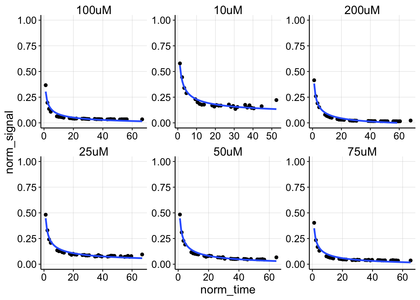

The decays actually look pretty similar between the different titration points. Let’s overlay all of them.

ggplot(swv_decays_norm %>% filter(rep != 0 | sub_rep != 1), aes(x = norm_time, 
    y = norm_signal)) + geom_point(aes(color = PHZadded)) + geom_smooth(method = "nls", 
    formula = y ~ b * (x)^-0.5 + a, method.args = list(start = c(b = 0.1, 
        a = 0)), se = F) + ylim(0, 1)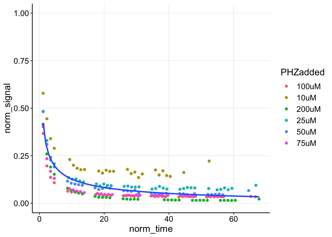

If we grab the coefficients from this fit they look like this:

swv_nls_fit <- nls(data = swv_decays_norm %>% filter(rep != 0 | 
    sub_rep != 1), formula = norm_signal ~ m * (norm_time)^-(1/2) + 
    a, start = list(a = 0, m = 0.1))

summary(swv_nls_fit)

## 
## Formula: norm_signal ~ m * (norm_time)^-(1/2) + a
## 
## Parameters:
##   Estimate Std. Error t value Pr(>|t|)    
## a -0.02333    0.00611  -3.818  0.00018 ***
## m  0.47534    0.02036  23.343  < 2e-16 ***
## ---
## Signif. codes:  0 '***' 0.001 '**' 0.01 '*' 0.05 '.' 0.1 ' ' 1
## 
## Residual standard error: 0.04889 on 199 degrees of freedom
## 
## Number of iterations to convergence: 1 
## Achieved convergence tolerance: 8.44e-09

Ok with the nonlinear \(m\) coefficient in hand we can compute \(D_m\):

\[D_m = \frac{D_{ap } t_s}{4 m^2}\] With the following parameters, let’s now look at \(D_m\) and \(D_{ap}\) for this biofilm.

t_s = 0.1  #not sure, total scan time is 2sec, and peak occurs at 1 sec so t_s must be <1sec
nls_m = 0.475
D_m = (D_ap * t_s)/(4 * nls_m^2)

paste("D_m =", D_m, "D_ap = ", D_ap)

## [1] "D_m = 5.24078493024045e-07 D_ap =  4.72980839954201e-06"

Ok, so we see about an order of magnitude difference between the estimated molecular diffusion coefficient, \(D_m\), and the estimated apparent electrochemical diffusion constant, \(D_{ap}\).

Discussion

Overall, I feel reasonably good about this analysis. The reason I re-did this experiment this way, was because I was concerned that the “equilibrium” PYO signal we saw was just background signal from the solution. By monitoring PYO as it decays out of the biofilm, we can be confident that the signal is coming from PYO in the actual biofilm.

That said, I would like to go back to the dataset from this experiment and try to background subtract the final GC to get a similar measure to the past experiments.

Most importantly, it seems to me that the SWV decays occur significantly more rapidly in this experiment than those from the past. This may be due to the use of the SWVfast, but I think it is most likely that it is caused by the repeated GC scans. By that I mean, that it’s possible that the large amount of PYO reduction that occurs during a GC scan actually influences the system, driving PYO out of the biofilm, since reduced PYO doesn’t bind DNA tightly.

If that is the case, we could just compare the \(D_{ap}\) from the GCs taken during the equilibration process to an uninterrupted SWV decay on the same biofilm?? However, I worry that this could be a bigger problem for our echem approach: When we estimate \(D_{ap}\) we assume that the \(D_{gc}\) is equivalent to \(D_{swv}\). Then because the two methods depend on \(D\) differently we can use that different dependence to estimate that parameter over a range of concentrations. What I worry is that in fact \(D_{gc} \approx D_{pyo_{red}}\) and that \(D_{swv} \approx D_{pyo_{ox}}\). That would be because SWV simply reduces the oxidized PYO near the electrode to generate a peak. Further, that reduction should be quick and hopefully doesn’t affect the whole pool of biofilm associated PYO? However, during GC, we typically quantify the collector current, which is poised at an oxidizing potential, therefore on some level it depends on \(PYO_{red}\) diffusing from the generator to the collector. We think that oxidized PYO is bound to DNA and its diffusion is slowed by it, but reduced PYO probably isn’t bound. If this is true and \(D_{pyo_{red}}\) is very different from \(D_{pyo_{ox}}\), then I think our measurements would be dominated by that. Therefore the difference between \(D_{ap}\) and \(D_m\) would be called into question, and our ability to estimate \(D_{ap}\) in the first place is questionable…

I’m not sure how to deal with this yet. This feels like yet another rabbit hole.

—–Edit——-

I believe that \(D_{gc}\) actually depends on both \(D_{pyo_{red}}\) and \(D_{pyo_{ox}}\). Let’s work backward from the collector electrode. The current at the collector electrode directly depends on \(D_{pyo_{red}}\). However, the \(PYO_{red}\) is actually produced at the generator electrode. The amount of \(PYO_{red}\) produced will depend on \(PYO_{ox}\) diffusing to the generator, aka \(D_{pyo_{ox}}\). Therefore, I think that \(D_{gc}\) directly depends on \(D_{pyo_{red}}\), but also indirectly depends on \(D_{pyo_{ox}}\). It would be ideal for us to assume that \(D_{pyo_{ox}} \approx D_{pyo_{red}}\), but that is probably not true in a biofilm full of eDNA. We don’t know how much slower \(D_{pyo_{ox}}\) may be, but if we believe that it is signficantly slower than \(D_{pyo_{red}}\) then the diffusion of \(PYO_{ox}\) to the generator electrode would become rate limiting. Therefore the measured GC current would still reflect \(D_{pyo_{ox}}\).

So, it may be true that the GCs are driving PYO out of the biofilm by reducing it, but I don’t actually think our approach is fundamentally flawed, because the GC probably mostly depends on \(D_{pyo_{ox}}\). Therefore we should compare these GCs with the pure SWV decays from other experiments.