Inter phenazine electron transfer in solution
Scott Saunders
09_17_19
Intro
Methods
Reduced phenazine prep
100uM of PCA, PYO and PCN were reduced in PBS 50 (50mL) in the survival assay chambers. Electrolysis was performed overnight and the expected color changes were observed. Reduced phenazines were transferred into stoppered serum bottles. Serum bottles were transferred to the anaerobic chamber housing the plate reader.
Pre electrolysis (left) & post electrolysis (right)
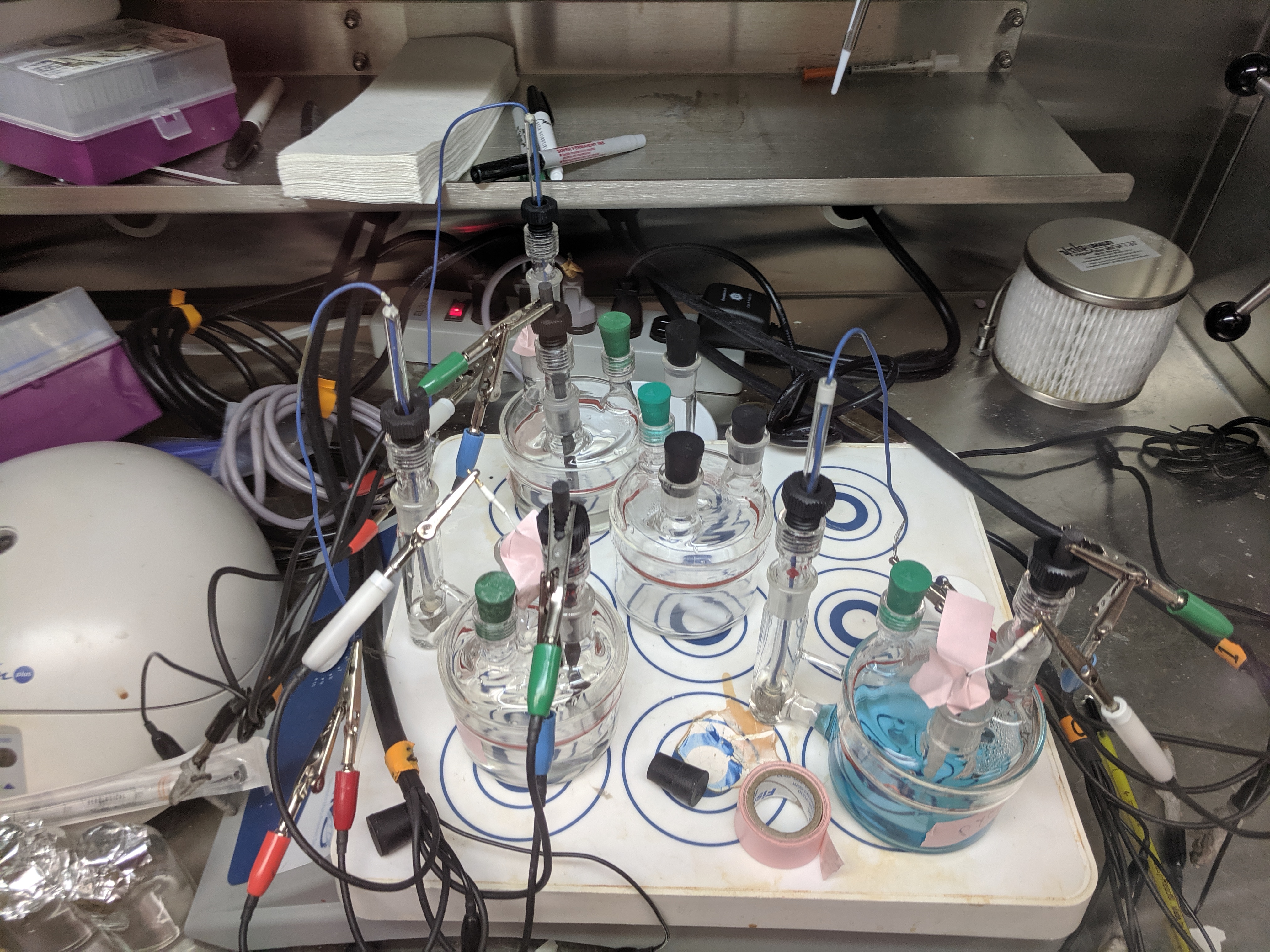
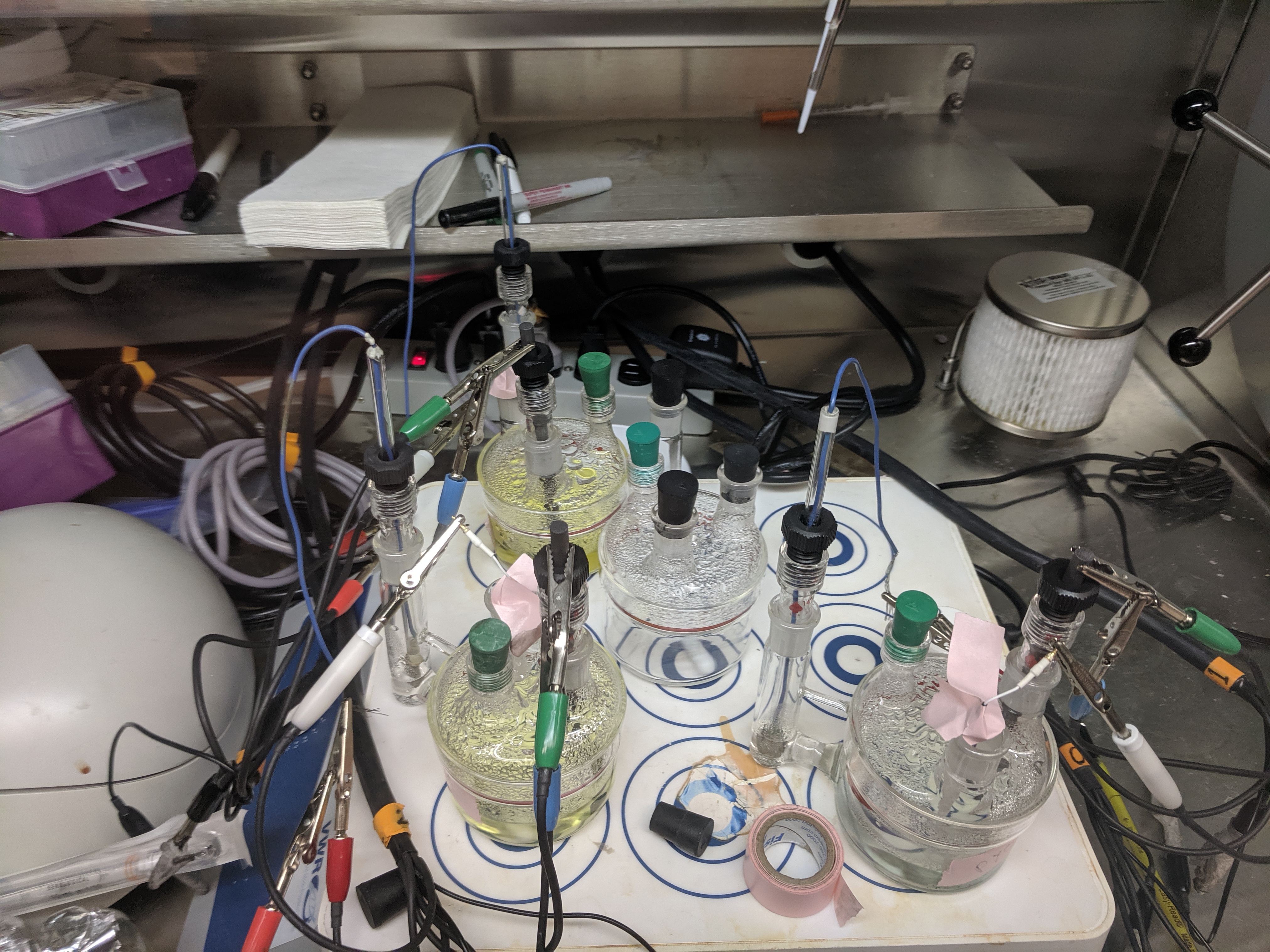
Clockwise from the bottom right the chambers are PYO, PCA and PCN.
Electrolysis curves (left) & serum bottles (right)
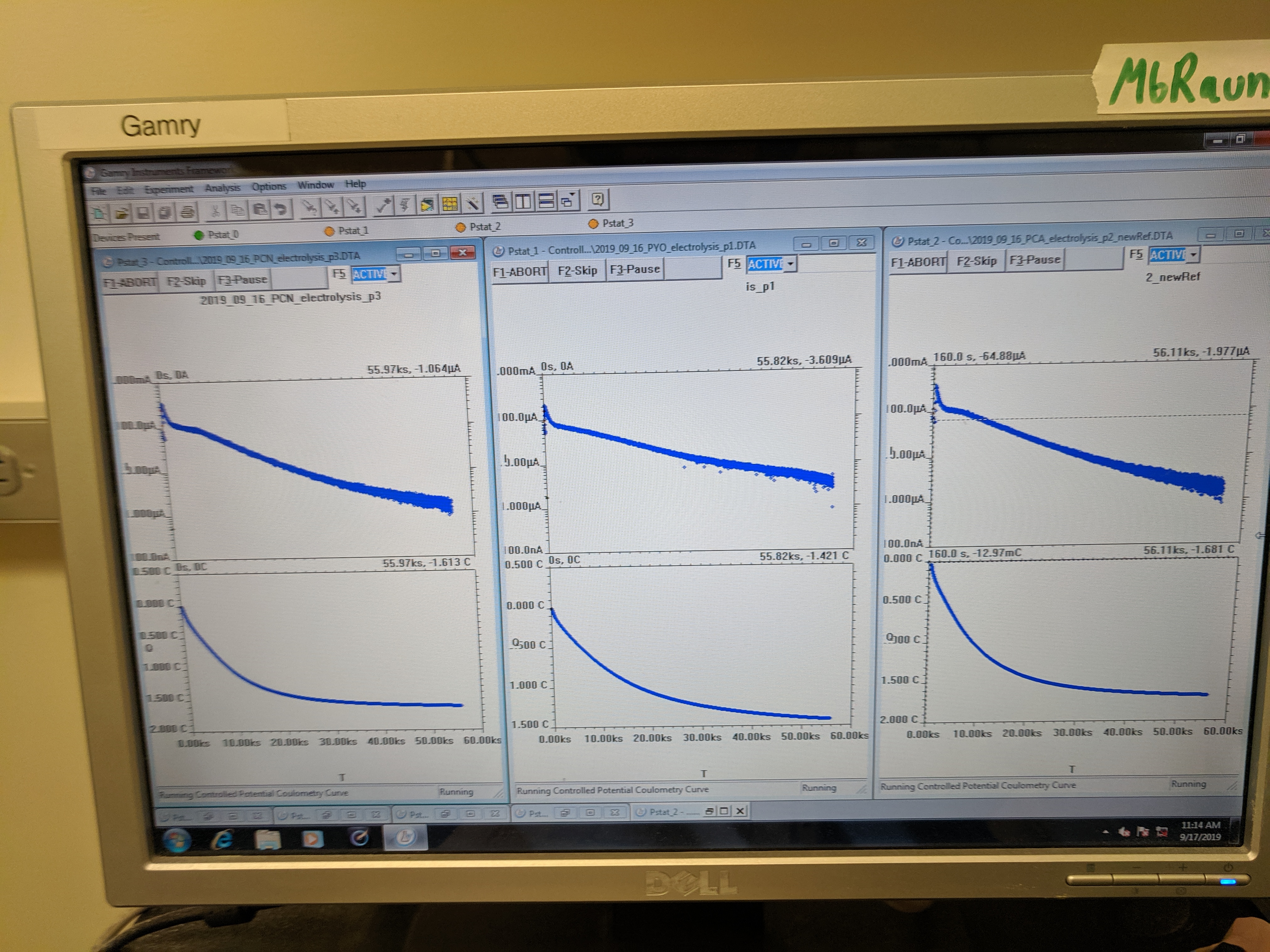
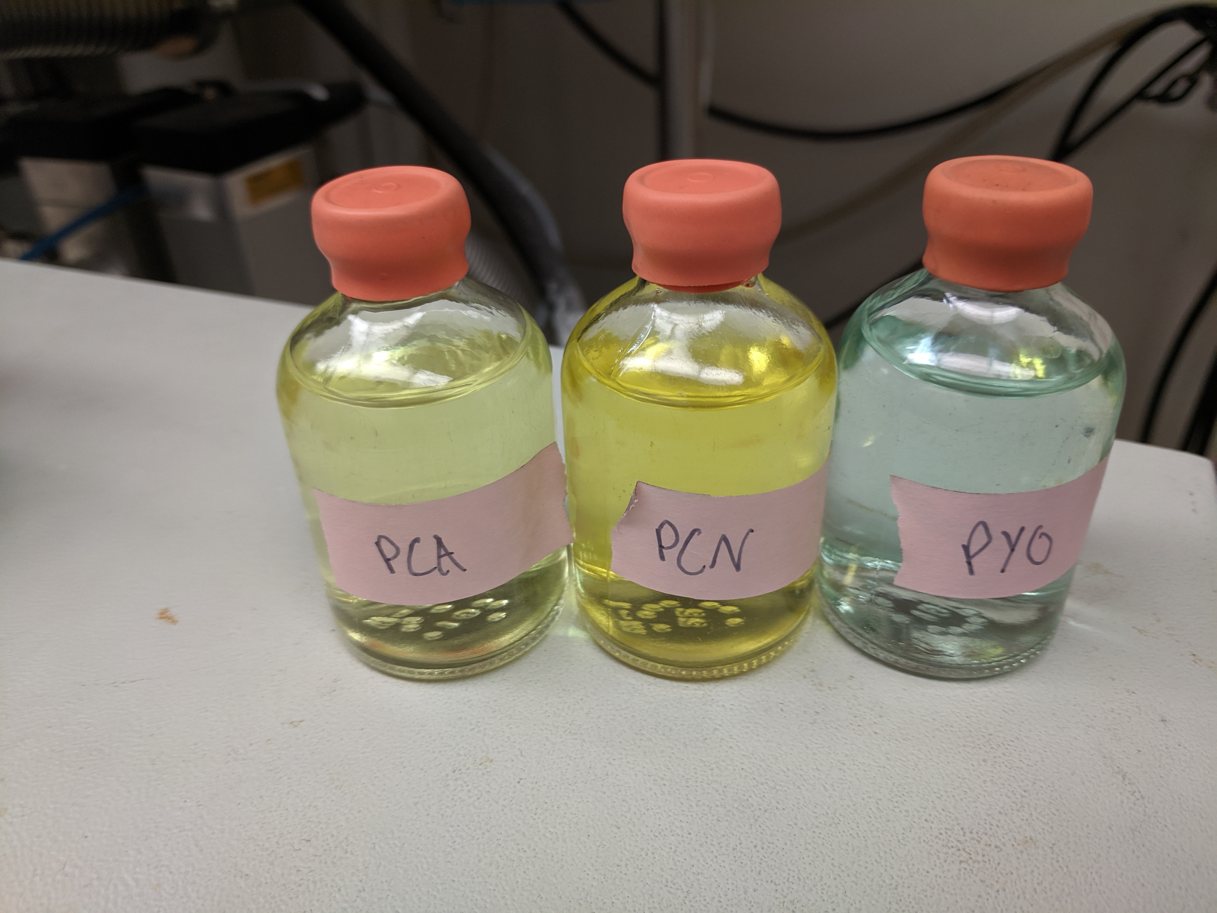
Electrolysis seemed to go to completion and the color changes remained in the serum bottles upon transfer to the other chamber.
Plate reader measurements
Black walled, clear bottomed fluorescence 96 well plates were stored in the chamber in advance. 1mL tubes of oxidized phenazines (100uM in PBS 50), and buffer (PBS 50), were transferred into the chamber the morning of and were shaken / pipetted repeatedly to remove oxygen.
Wells were measured in two fluorescence channels 360/40ex,460/40 em and 360/40ex, 528/40 em and absorbance scans were taken from 300nm - 700nm in increments of 10nm. Wells were scanned with oxidized phenazines before mixing, and then repeatedly scanned in a timecourse following mixing.
Experimental design
Mixing 75uL of reduced phz (or buffer) with 75uL of oxidized phz (or buffer)
1. Buffer
- Buffer –> Buffer
- Buffer –> \(PCA_{ox}\)
- Buffer –> \(PCN_{ox}\)
- Buffer –> \(PYO_{ox}\)
2. \(PCA_{red}\)
- \(PCA_{red}\) –> Buffer
- \(PCA_{red}\) –> \(PYO_{ox}\)
- \(PCA_{red}\) –> \(PCN_{ox}\)
3. \(PCN_{red}\)
- \(PCN_{red}\) –> Buffer
- \(PCN_{red}\) –> \(PYO_{ox}\)
- \(PCN_{red}\) –> \(PCA_{ox}\)
4. \(PYO_{red}\)
- \(PYO_{red}\) –> Buffer
- \(PYO_{red}\) –> \(PCA_{ox}\)
- \(PYO_{red}\) –> \(PCN_{ox}\)
In this way we acquired spectra in the measured channels for all of the oxidized and reduced phenazines in isolation and in combination. Well conditions were repeated in triplicate.
The actual setup and plate reader program was to do the PBS controls first with oxidized and reduced phenazines (wells B1-B6). The plate reader program was to take an absorbance spectra, then do a kinetic run for 2min monitoring all the abs and fluor wavelenghts, then taking another absorbance spectra.
After the controls, then I setup wells C1-C6 with PCN_ox (C1-C3) and PYO_ox (C4 - C6) and added PCA_red. Then I did PCN_red with PCA_ox and PYO_ox in wells D1-D6, followed by PYO_red with PCA_ox and PCN_ox (E1-E6). Finally I ran the same plate reader program on the entire plate. Therefore there are 4 spectra and two kinetic runs per well. Howerver, as you will see, we only need to look at the first spectra and the first kinetic read.
Results
First let’s just look at the metadata telling us which experiment occurred in which well:
library(tidyverse)
library(cowplot)
library(viridis)
library(knitr)
library(kableExtra)


knitr::opts_chunk$set(tidy.opts=list(width.cutoff=60),tidy=TRUE, echo = TRUE, message=FALSE, warning=FALSE, fig.align="center")

source("../../IDA/tools/plotting_tools.R")

theme_set(theme_1())
metadata <- read_csv("data/2019_09_17_solution_ET_well_metadata.csv") %>%
mutate(exp = ifelse(red == "PBS" | ox == "PBS", "ref", "exp"))
metadata %>% kable() %>% kable_styling(bootstrap_options = "condensed") %>%
scroll_box(width = "100%", height = "400px")| well | red | ox | red_ox | rep | exp |
|---|---|---|---|---|---|
| B1 | PBS | PCA | PBS_PCA | 1 | ref |
| B2 | PBS | PCN | PBS_PCN | 1 | ref |
| B3 | PBS | PYO | PBS_PYO | 1 | ref |
| B4 | PCA | PBS | PCA_PBS | 1 | ref |
| B5 | PCN | PBS | PCN_PBS | 1 | ref |
| B6 | PYO | PBS | PYO_PBS | 1 | ref |
| C1 | PCA | PCN | PCA_PCN | 1 | exp |
| C2 | PCA | PCN | PCA_PCN | 2 | exp |
| C3 | PCA | PCN | PCA_PCN | 3 | exp |
| C4 | PCA | PYO | PCA_PYO | 1 | exp |
| C5 | PCA | PYO | PCA_PYO | 2 | exp |
| C6 | PCA | PYO | PCA_PYO | 3 | exp |
| D1 | PCN | PCA | PCN_PCA | 1 | exp |
| D2 | PCN | PCA | PCN_PCA | 2 | exp |
| D3 | PCN | PCA | PCN_PCA | 3 | exp |
| D4 | PCN | PYO | PCN_PYO | 1 | exp |
| D5 | PCN | PYO | PCN_PYO | 2 | exp |
| D6 | PCN | PYO | PCN_PYO | 3 | exp |
| E1 | PYO | PCA | PYO_PCA | 1 | exp |
| E2 | PYO | PCA | PYO_PCA | 2 | exp |
| E3 | PYO | PCA | PYO_PCA | 3 | exp |
| E4 | PYO | PCN | PYO_PCN | 1 | exp |
| E5 | PYO | PCN | PYO_PCN | 2 | exp |
| E6 | PYO | PCN | PYO_PCN | 3 | exp |
| A4 | PBS | PBS | PBS_PBS | 1 | ref |
| A5 | PBS | PBS | PBS_PBS | 2 | ref |
| A6 | PBS | PBS | PBS_PBS | 3 | ref |
Reference Spectra / values
Let’s start by looking at the reference spectra for the oxidized and reduced phenazines.
df_spectra <- read_csv("data/2019_09_17_solution_ET_abs_spectra_1.csv",
    skip = 1) %>% gather(key = "well", value = "intensity", -Wavelength)

df_spectra_meta <- left_join(df_spectra, metadata, by = c("well")) %>%
    mutate(phz = case_when(red == "PYO" | ox == "PYO" ~ "PYO",
        red == "PCA" | ox == "PCA" ~ "PCA", red == "PCN" | ox ==
            "PCN" ~ "PCN", red_ox == "PBS_PBS" & rep == 1 ~ "PCA",
        red_ox == "PBS_PBS" & rep == 2 ~ "PCN", red_ox == "PBS_PBS" &
            rep == 3 ~ "PYO")) %>% mutate(phz_redox = ifelse(red ==
    "PBS", "phz_ox", "phz_red"))
ggplot(df_spectra_meta %>% filter(rep == 1) %>% filter(exp ==
"ref" & red_ox != "PBS_PBS"), aes(x = Wavelength, color = phz_redox,
group = red_ox)) + geom_vline(xintercept = c(310, 360, 500,
690), color = "gray", linetype = 2, alpha = 0.4) + geom_path(data = df_spectra_meta %>%
filter(red_ox == "PBS_PBS"), aes(x = Wavelength, y = intensity),
color = "gray") + geom_path(aes(y = intensity), size = 1) +
facet_wrap(~phz, scales = "free") + labs(color = NULL, y = "Absorbance")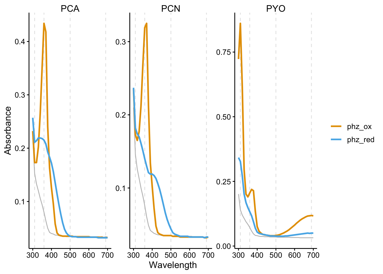
Gray is the PBS background and the dashed gray lines are the wavelengths I measured over time (not including the fluorescence channels).
Comparing spectra
Now let’s put the spectra together for each experimental well. Ideally we’d like to compare the experimentally observed spectrum to the oxidized and reduced phenazines added to the well to see how the reaction proceeded. We need to wrangle some of the data to put that all together, but now we can explore each condition:
df_ref_1 <- left_join(df_spectra_meta %>% filter(exp == "exp"),
    df_spectra_meta %>% filter(exp == "ref") %>% select(Wavelength,
        well, intensity, red, ox, red_ox), by = c("red", "Wavelength"),
    suffix = c("", "_phz1_red"))

df_ref_2 <- left_join(df_ref_1, df_spectra_meta %>% filter(exp ==
    "ref") %>% select(Wavelength, well, intensity, red, ox, red_ox),
    by = c(red = "ox", "Wavelength"), suffix = c("", "_phz1_ox"))

df_ref_3 <- left_join(df_ref_2, df_spectra_meta %>% filter(exp ==
    "ref") %>% select(Wavelength, well, intensity, red, ox, red_ox),
    by = c("ox", "Wavelength"), suffix = c("", "_phz2_ox"))

df_ref_4 <- left_join(df_ref_3, df_spectra_meta %>% filter(exp ==
    "ref") %>% select(Wavelength, well, intensity, red, ox, red_ox),
    by = c(ox = "red", "Wavelength"), suffix = c("", "_phz2_red"))


legend_segments <- tibble(x = c(500, 500, 500, 500), xend = c(550,
    550, 550, 550), xlabel = c(525, 525, 525, 525), y = c(0.4,
    0.3, 0.2, 0.1), color = c("red", "red", "blue", "blue"),
    linetype = c(1, 2, 1, 2), label = c("PHZ 1 reduced (init)",
        "PHZ 1 oxidized (final)", "PHZ 2 oxidized (init)", "PHZ 2 reduced (final)"))


color = c("red", "red", "blue", "blue")
linetype = c(1, 2, 1, 2)

spectra_legend <- geom_segment(data = legend_segments, aes(x = x,
    xend = xend, y = y, yend = y), color = color, linetype = linetype,
    size = 1)

legend_labs <- geom_text(data = legend_segments, aes(x = xlabel,
    y = y, label = label), nudge_y = 0.05)
\(PCA_{red} + PYO_{ox}\)
ggplot(df_ref_4 %>% filter(rep == 1 & red_ox == "PCA_PYO"), aes(x = Wavelength)) +
    geom_path(aes(y = intensity_phz1_red), color = "red", linetype = 1,
        size = 1) + geom_path(aes(y = intensity_phz1_ox), color = "red",
    linetype = 2, size = 1) + geom_path(aes(y = intensity_phz2_ox),
    color = "blue", linetype = 1, size = 1) + geom_path(aes(y = intensity_phz2_red),
    color = "blue", linetype = 2, size = 1) + geom_path(aes(y = intensity),
    size = 1) + facet_wrap(~red_ox, scales = "free") + spectra_legend +
    legend_labs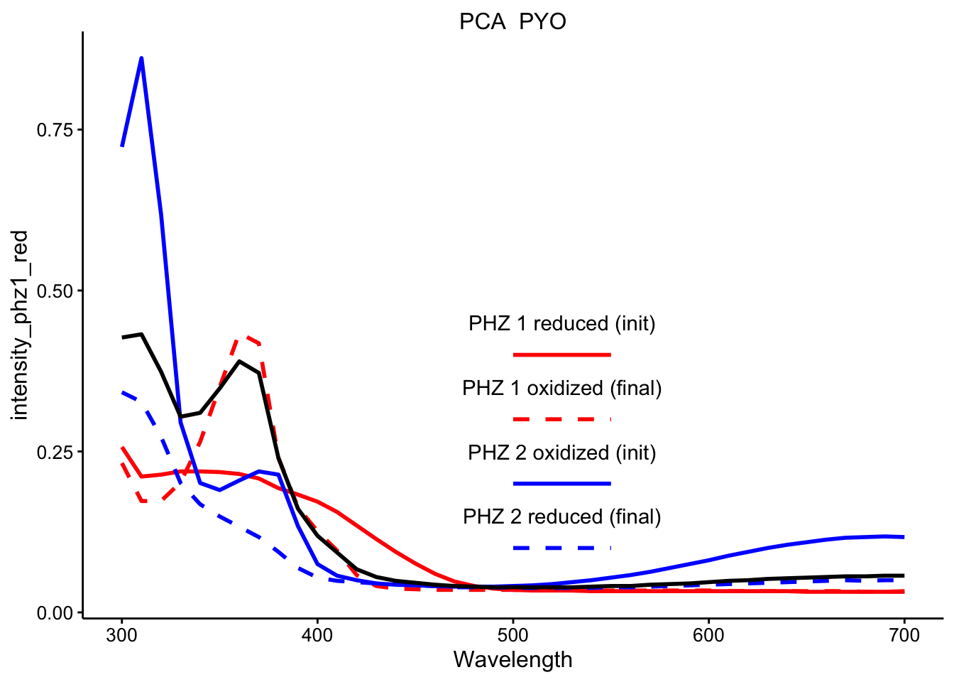
\(PCN_{red} + PYO_{ox}\)
ggplot(df_ref_4 %>% filter(rep == 1 & red_ox == "PCN_PYO"), aes(x = Wavelength)) +
    geom_path(aes(y = intensity_phz1_red), color = "red", linetype = 1,
        size = 1) + geom_path(aes(y = intensity_phz1_ox), color = "red",
    linetype = 2, size = 1) + geom_path(aes(y = intensity_phz2_ox),
    color = "blue", linetype = 1, size = 1) + geom_path(aes(y = intensity_phz2_red),
    color = "blue", linetype = 2, size = 1) + geom_path(aes(y = intensity),
    size = 1) + facet_wrap(~red_ox, scales = "free") + spectra_legend +
    legend_labs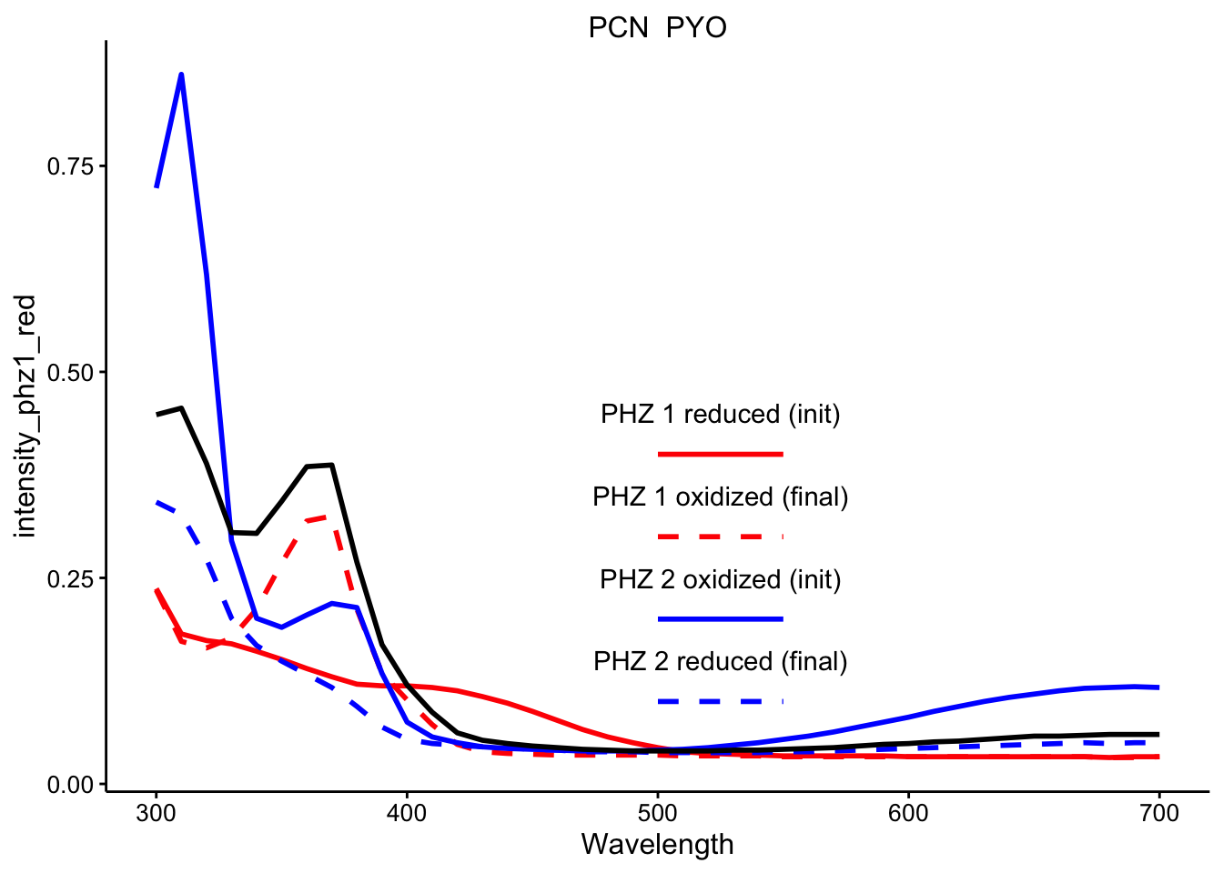
\(PYO_{red} + PCA_{ox}\)
ggplot(df_ref_4 %>% filter(rep == 1 & red_ox == "PYO_PCA"), aes(x = Wavelength)) +
    geom_path(aes(y = intensity_phz1_red), color = "red", linetype = 1,
        size = 1) + geom_path(aes(y = intensity_phz1_ox), color = "red",
    linetype = 2, size = 1) + geom_path(aes(y = intensity_phz2_ox),
    color = "blue", linetype = 1, size = 1) + geom_path(aes(y = intensity_phz2_red),
    color = "blue", linetype = 2, size = 1) + geom_path(aes(y = intensity),
    size = 1) + facet_wrap(~red_ox, scales = "free") + spectra_legend +
    legend_labs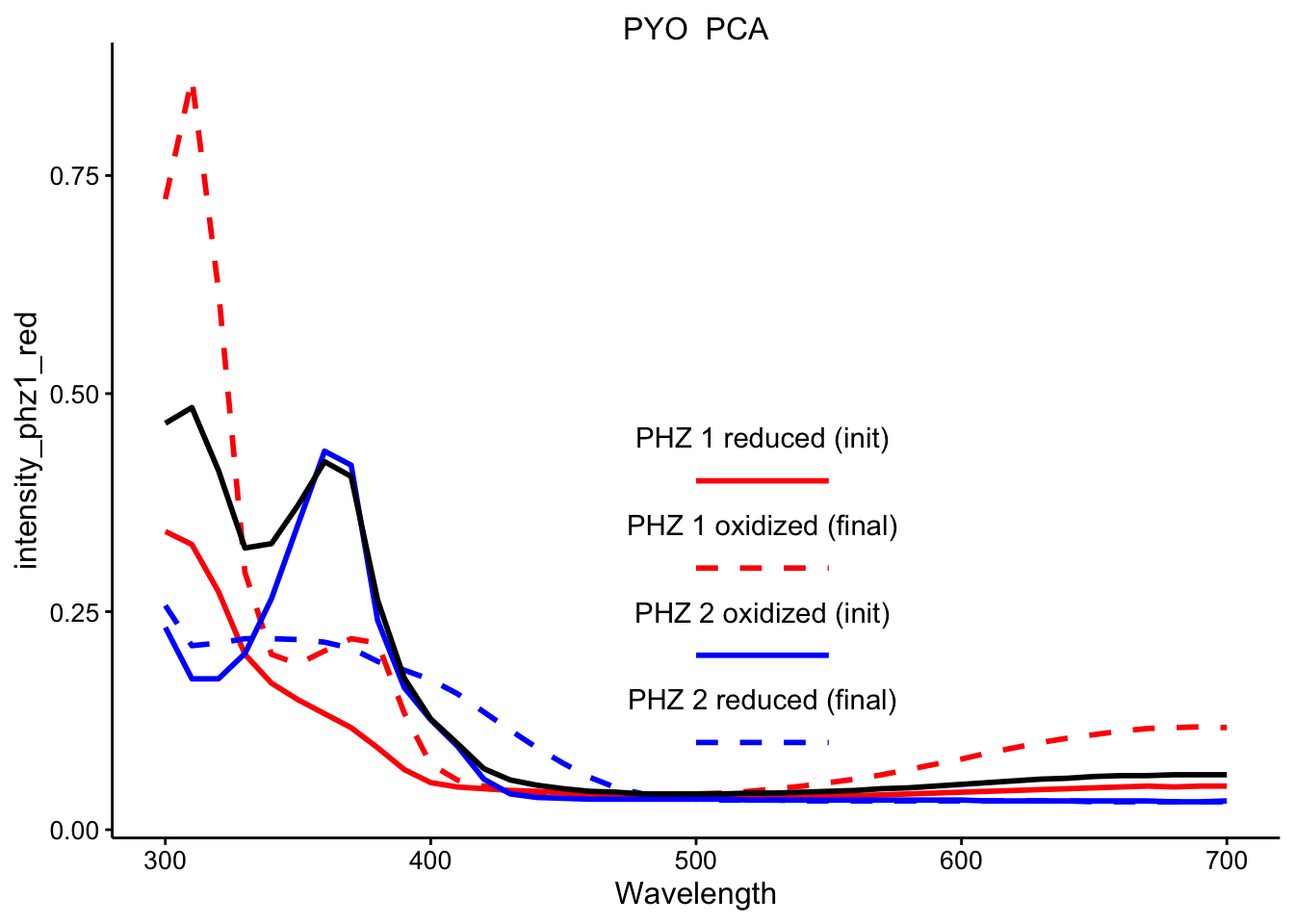
\(PYO_{red} + PCN_{ox}\)
ggplot(df_ref_4 %>% filter(rep == 1 & red_ox == "PYO_PCN"), aes(x = Wavelength)) +
    geom_path(aes(y = intensity_phz1_red), color = "red", linetype = 1,
        size = 1) + geom_path(aes(y = intensity_phz1_ox), color = "red",
    linetype = 2, size = 1) + geom_path(aes(y = intensity_phz2_ox),
    color = "blue", linetype = 1, size = 1) + geom_path(aes(y = intensity_phz2_red),
    color = "blue", linetype = 2, size = 1) + geom_path(aes(y = intensity),
    size = 1) + facet_wrap(~red_ox, scales = "free") + spectra_legend +
    legend_labs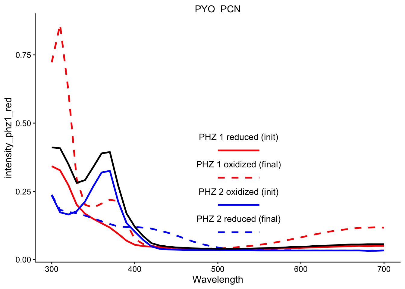
\(PCN_{red} + PCA_{ox}\)
ggplot(df_ref_4 %>% filter(rep == 1 & red_ox == "PCN_PCA"), aes(x = Wavelength)) +
    geom_path(aes(y = intensity_phz1_red), color = "red", linetype = 1,
        size = 1) + geom_path(aes(y = intensity_phz1_ox), color = "red",
    linetype = 2, size = 1) + geom_path(aes(y = intensity_phz2_ox),
    color = "blue", linetype = 1, size = 1) + geom_path(aes(y = intensity_phz2_red),
    color = "blue", linetype = 2, size = 1) + geom_path(aes(y = intensity),
    size = 1) + facet_wrap(~red_ox, scales = "free") + spectra_legend +
    legend_labs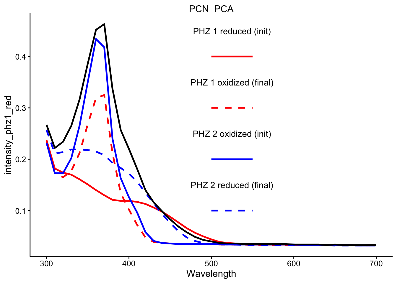
\(PCA_{red} + PCN_{ox}\)
ggplot(df_ref_4 %>% filter(rep == 1 & red_ox == "PCA_PCN"), aes(x = Wavelength)) +
    geom_path(aes(y = intensity_phz1_red), color = "red", linetype = 1,
        size = 1) + geom_path(aes(y = intensity_phz1_ox), color = "red",
    linetype = 2, size = 1) + geom_path(aes(y = intensity_phz2_ox),
    color = "blue", linetype = 1, size = 1) + geom_path(aes(y = intensity_phz2_red),
    color = "blue", linetype = 2, size = 1) + geom_path(aes(y = intensity),
    size = 1) + facet_wrap(~red_ox, scales = "free") + spectra_legend +
    legend_labs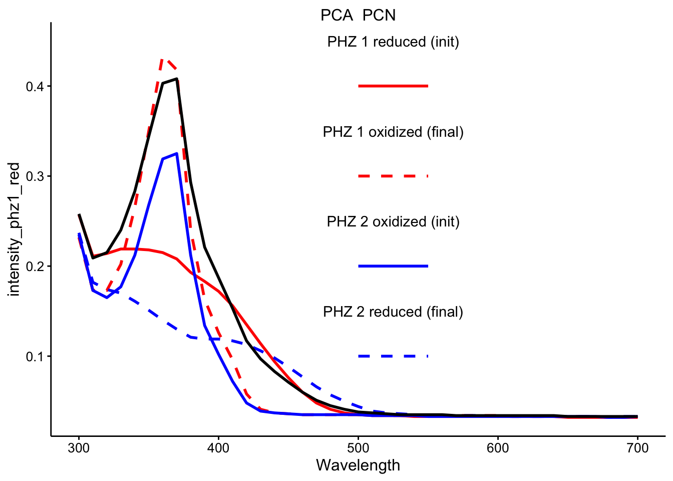
Kinetic run
df_kin <- read_csv("data/2019_09_17_solution_ET_init_kinetic_reads.csv",
    skip = 1, ) %>% select(-`Kinetic read`) %>% gather(key = "well",
    value = "intensity", -minutes, -wavelength)

df_kin <- left_join(df_kin, metadata, by = c("well"))
Looking at these kinetic reads over the initial 2 minutes (following mixing, starting protocol and abs spectra), it seems like we aren’t observing a lot of change over this timescale. I think this means that the reactions either happen fast, before the measurement, or they are not going / proceeding very slowly.
em460
ggplot(df_kin %>% filter(wavelength == "em460"), aes(x = minutes,
    y = intensity)) + geom_point() + geom_smooth(method = "lm",
    se = F) + facet_grid(red ~ ox)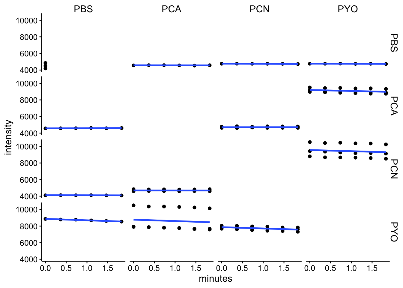
em528
ggplot(df_kin %>% filter(wavelength == "em528"), aes(x = minutes,
    y = intensity)) + geom_point() + geom_smooth(method = "lm",
    se = F) + facet_grid(red ~ ox)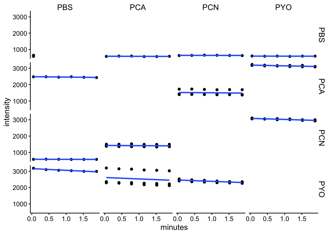
abs310
ggplot(df_kin %>% filter(wavelength == "abs310"), aes(x = minutes,
    y = intensity)) + geom_point() + geom_smooth(method = "lm",
    se = F) + facet_grid(red ~ ox)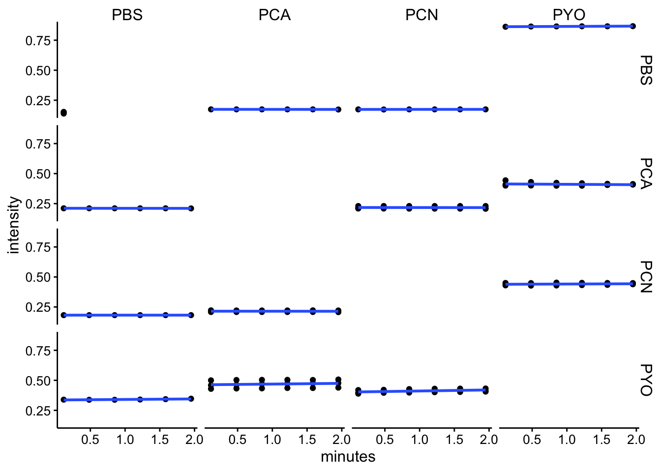
abs360
ggplot(df_kin %>% filter(wavelength == "abs360"), aes(x = minutes,
    y = intensity)) + geom_point() + geom_smooth(method = "lm",
    se = F) + facet_grid(red ~ ox)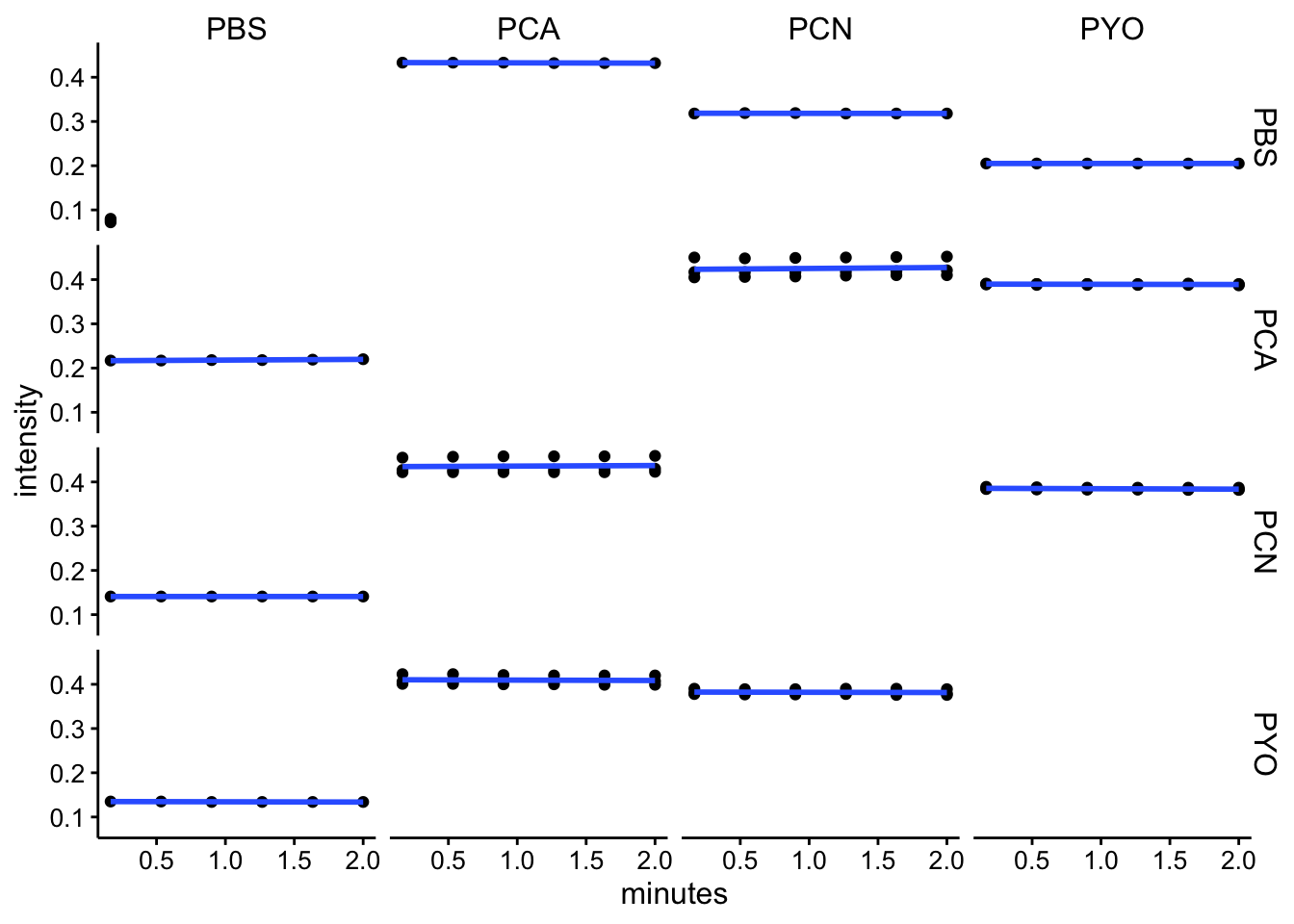
abs690
ggplot(df_kin %>% filter(wavelength == "abs690"), aes(x = minutes,
    y = intensity)) + geom_point() + geom_smooth(method = "lm",
    se = F) + facet_grid(red ~ ox)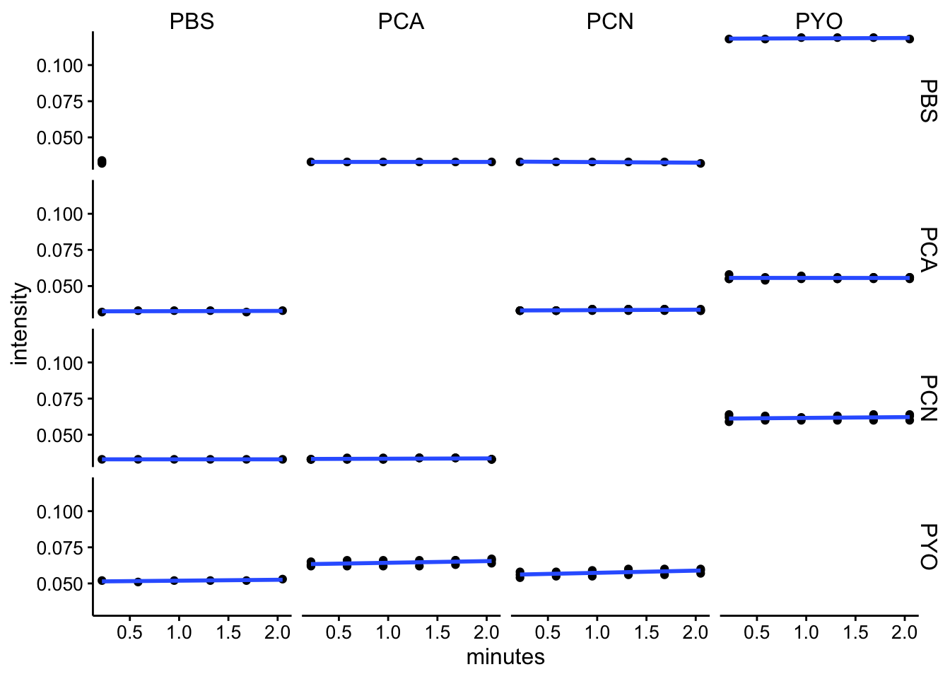
abs500
ggplot(df_kin %>% filter(wavelength == "abs500"), aes(x = minutes,
    y = intensity)) + geom_point() + geom_smooth(method = "lm",
    se = F) + facet_grid(red ~ ox)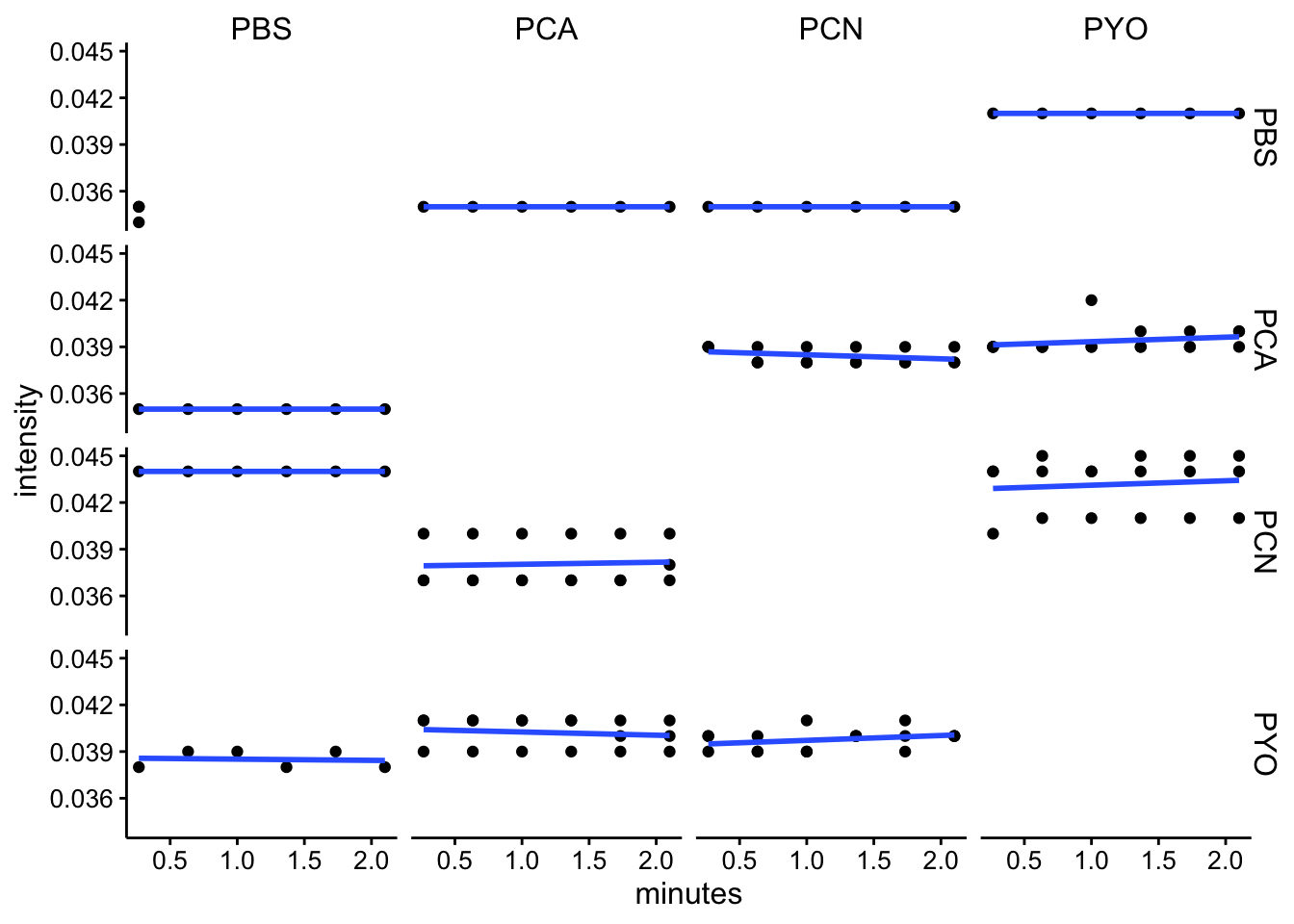
Quantifying and predicting rxns
Now that it doesn’t matter which point values we take from the kinetic run, let’s just average the kinetic run values for each well and take a look:
df_per_rep <- df_kin %>% group_by(wavelength, red, ox, red_ox,
    rep) %>% summarise(int_per_rep = mean(intensity, na.rm = T),
    std_per_rep = sd(intensity, na.rm = T)) %>% mutate(std_per_rep = ifelse(is.na(std_per_rep),
    0, std_per_rep))


ggplot(df_per_rep, aes(x = red_ox, y = int_per_rep)) + geom_pointrange(aes(ymin = int_per_rep -
    2 * std_per_rep, ymax = int_per_rep + 2 * std_per_rep)) +
    facet_wrap(~wavelength, scales = "free")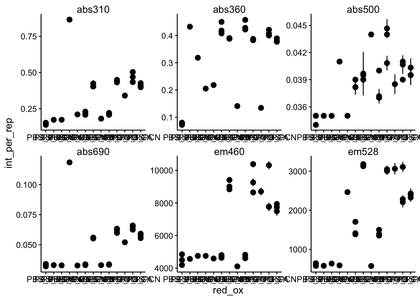
Ok, hard to read, but the point is there are different values and the error bars are small, because the kinetic reads were pretty much all the same. Note that error bars are 2 standard deviations aka approximately a 95% confidence interval. Now let’s average the triplicates from each condition:
df_per_cond <- df_per_rep %>% group_by(wavelength, red, ox, red_ox) %>%
    summarise(int_per_cond = mean(int_per_rep), std_per_cond = sd(int_per_rep)) %>%
    mutate(std_per_cond = ifelse(is.na(std_per_cond), 0, std_per_cond))


ggplot(df_per_cond, aes(x = red_ox, y = int_per_cond)) + geom_hline(data = df_per_cond %>%
    filter(red_ox == "PBS_PBS"), aes(yintercept = int_per_cond),
    color = "gray") + geom_pointrange(aes(ymin = int_per_cond -
    2 * std_per_cond, ymax = int_per_cond + 2 * std_per_cond)) +
    facet_wrap(~wavelength, scales = "free") + ylim(0, NA)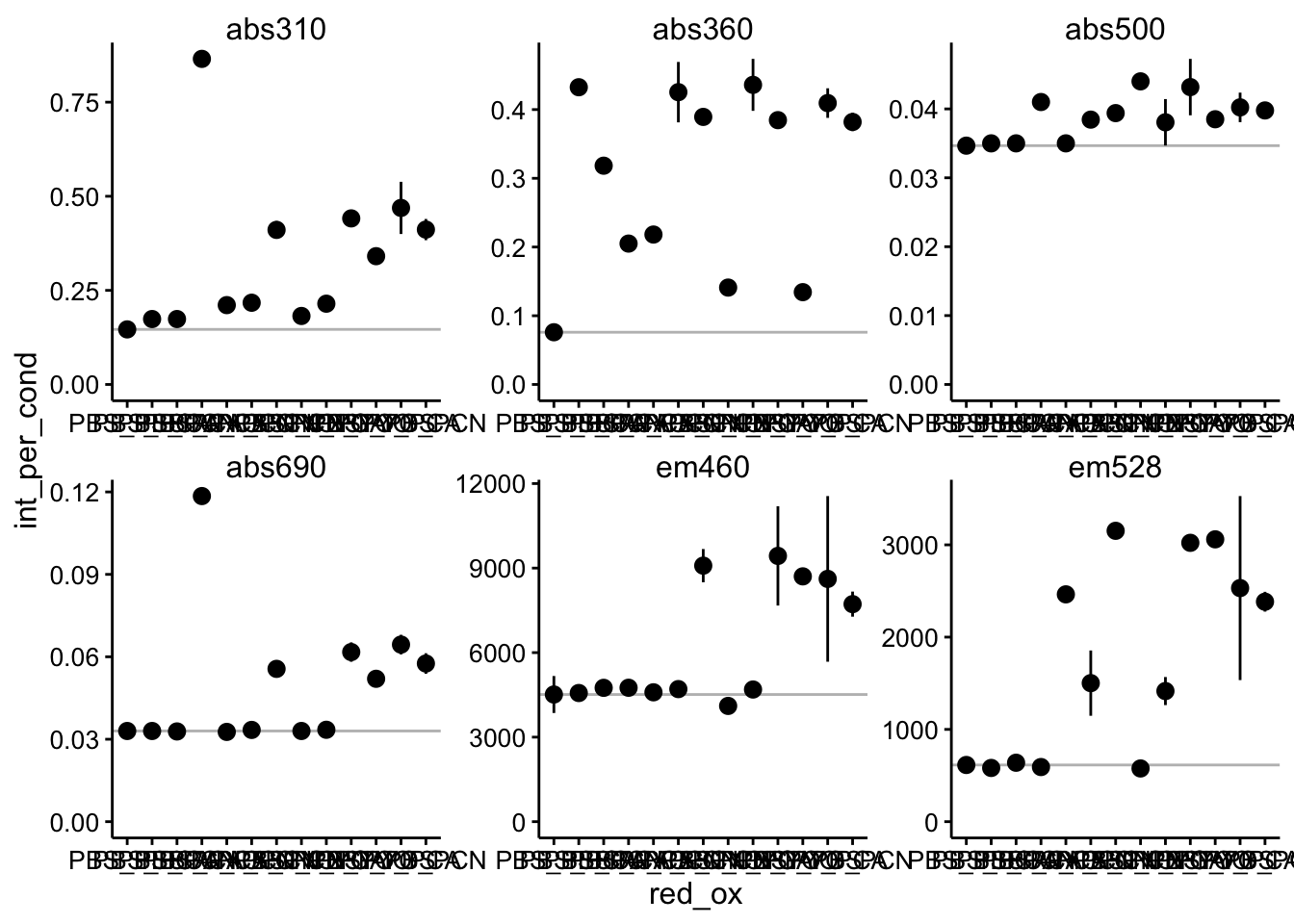
Ok, here you can see that error bars are a little bigger to accomodate the triplicate wells. I have also plotted in a gray line the value of the PBS only control. This gives us a good idea of what the background reading is without any phenazine. Let’s go ahead and subtract out that background - this is equivalent to blanking a spec etc.
df_bg_sub <- df_per_cond %>% group_by(wavelength) %>% mutate(bg = ifelse(red_ox ==
    "PBS_PBS", int_per_cond, NA)) %>% mutate(bg_sub = int_per_cond -
    mean(bg, na.rm = T))

ggplot(df_bg_sub, aes(x = red_ox, y = bg_sub)) + geom_hline(data = df_bg_sub %>%
    filter(red_ox == "PBS_PBS"), aes(yintercept = bg_sub), color = "gray") +
    geom_pointrange(aes(ymin = bg_sub - 2 * std_per_cond, ymax = bg_sub +
        2 * std_per_cond)) + facet_wrap(~wavelength, scales = "free")  # + ylim(0,NA)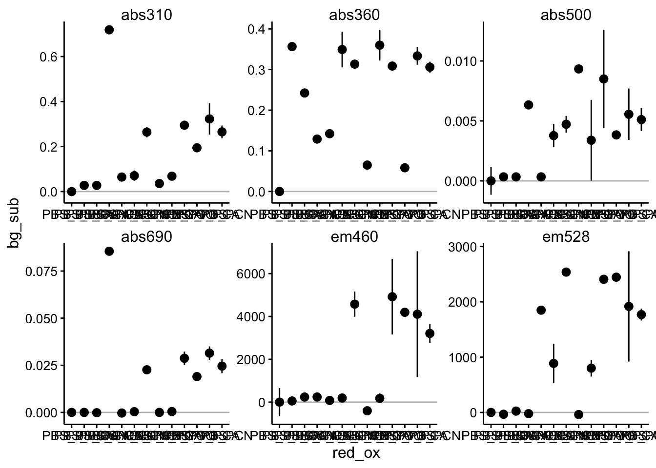
Beautiful, now these should be the intensities of the actual phenazines we were trying to measure.
Now what I’m going to do is setup the data so that we can actually predict the initial and final intensities for each well. For example, the \(PCA_{red} + PYO_{ox}\) condition should start with the abs690 of \(690_{PCA_{red}} + 690_{PYO_{ox}}\) and if the redox reaction proceeds the final values should be \(690_{PCA_{ox}} + 690_{PYO_{red}}\). Now you can look at the predictions vs. the experimental values for each of the conditions and channels:
bg_sub_refs <- df_bg_sub %>% filter(str_detect(red_ox, "PBS")) %>%
    filter(red_ox != "PBS_PBS")

bg_sub_phz1_red <- left_join(df_bg_sub %>% filter(!str_detect(red_ox,
    "PBS")), bg_sub_refs, by = c("wavelength", "red"), suffix = c("",
    "_from_phz1_red"))

bg_sub_phz1_ox <- left_join(bg_sub_phz1_red, bg_sub_refs, by = c("wavelength",
    red = "ox"), suffix = c("", "_from_phz1_ox"))

bg_sub_phz2_ox <- left_join(bg_sub_phz1_ox, bg_sub_refs, by = c("wavelength",
    "ox"), suffix = c("", "_from_phz2_ox"))

bg_sub_phz2_red <- left_join(bg_sub_phz2_ox, bg_sub_refs, by = c("wavelength",
    ox = "red"), suffix = c("", "_from_phz2_red"))

bg_sub_redox <- bg_sub_phz2_red %>% mutate(pred_init = bg_sub_from_phz1_red +
    bg_sub_from_phz2_ox, pred_final = bg_sub_from_phz1_ox + bg_sub_from_phz2_red)

# red_ox_labs =
# c('PCA[red]~'+\n'*PCN[ox]',''PCA[red]+\nPYO[ox]'',''PCN[red]+\nPCA[ox]'',''PCN[red]+\nPYO[ox]'',''PYO[red]+\nPCA[ox]'',
# ''PYO[red]+\nPCN[ox]'')

red_ox_labs = c("PCA_red+\nPCN_ox", "PCA_red+\nPYO_ox", "PCN_red+\nPCA_ox",
    "PCN_red+\nPYO_ox", "PYO_red+\nPCA_ox", "PYO_red+\nPCN_ox")


# red_ox_labs = c(expression(PCA[red]~'+\n'PCN[ox]))
Note that the red dot is the initial prediction, blue dot is the final prediction, and the black pointrange (95% CI) is the experimental values.
Predicted intensities
abs 310
ggplot(bg_sub_redox %>% filter(wavelength == "abs310"), aes(x = red_ox)) +
    geom_point(aes(y = pred_init), color = "red") + geom_point(aes(y = pred_final),
    color = "blue") + geom_pointrange(aes(y = bg_sub, ymin = bg_sub -
    2 * std_per_cond, ymax = bg_sub + 2 * std_per_cond), shape = 21) +
    facet_wrap(~wavelength, scales = "free") + scale_x_discrete(labels = red_ox_labs,
    name = NULL) + theme(axis.text.x = element_text(size = 12)) +
    labs(y = "Predicted intensity")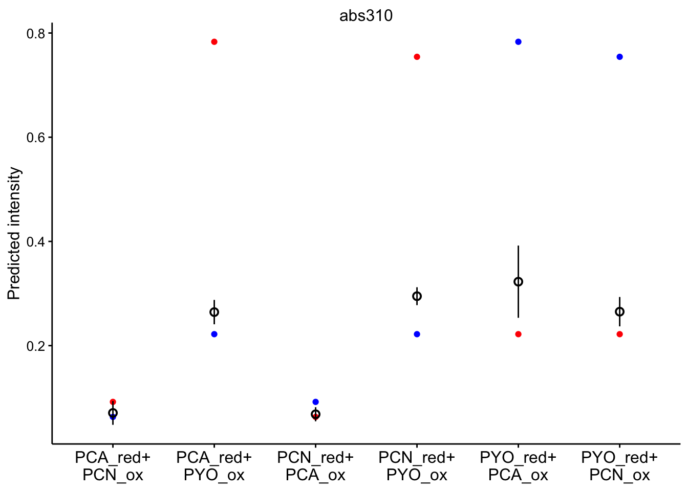
abs 360
ggplot(bg_sub_redox %>% filter(wavelength == "abs360"), aes(x = red_ox)) +
    geom_point(aes(y = pred_init), color = "red") + geom_point(aes(y = pred_final),
    color = "blue") + geom_pointrange(aes(y = bg_sub, ymin = bg_sub -
    2 * std_per_cond, ymax = bg_sub + 2 * std_per_cond), shape = 21) +
    facet_wrap(~wavelength, scales = "free") + scale_x_discrete(labels = red_ox_labs,
    name = NULL) + theme(axis.text.x = element_text(size = 12)) +
    labs(y = "Predicted intensity")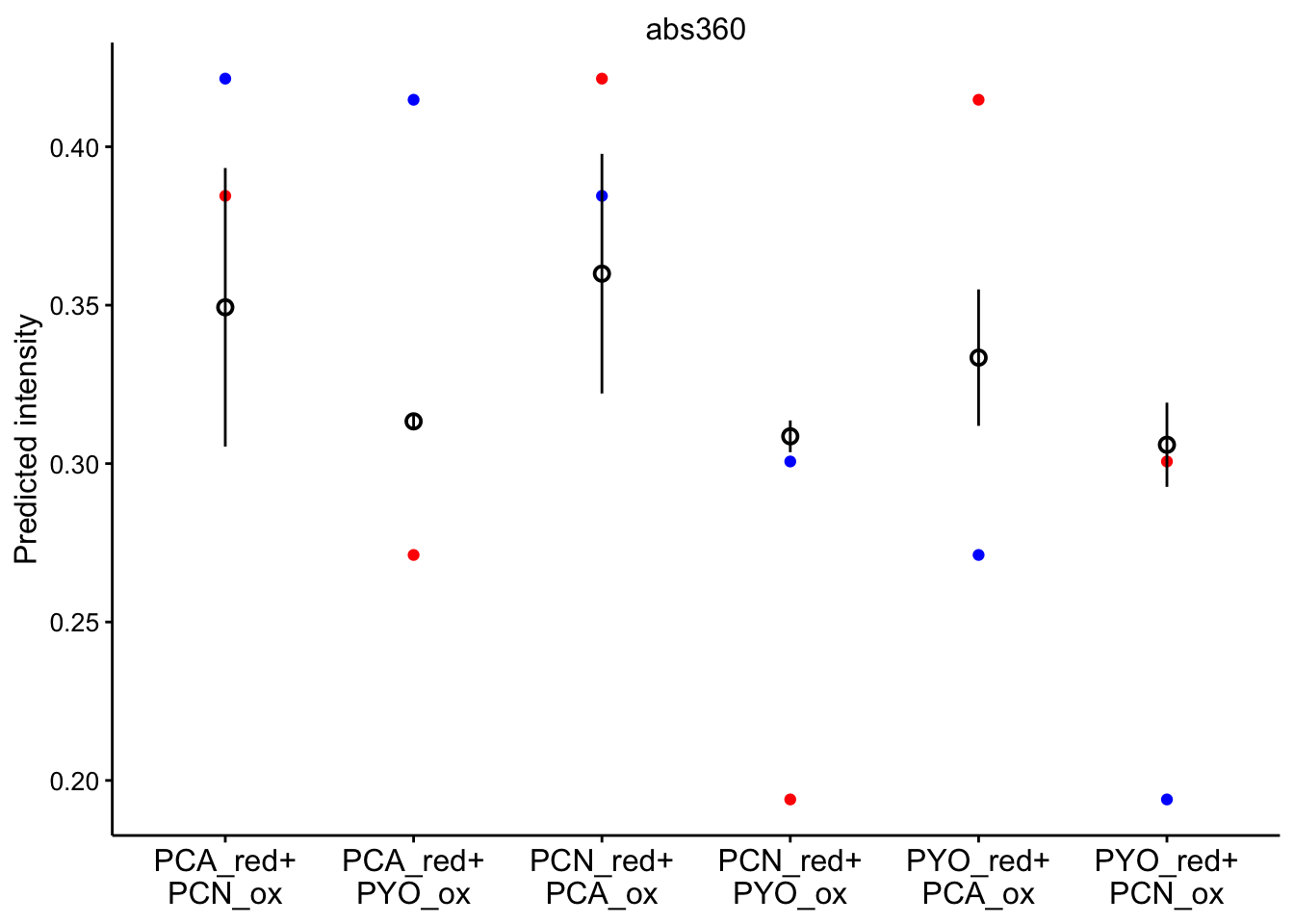
abs 690
ggplot(bg_sub_redox %>% filter(wavelength == "abs690"), aes(x = red_ox)) +
    geom_point(aes(y = pred_init), color = "red") + geom_point(aes(y = pred_final),
    color = "blue") + geom_pointrange(aes(y = bg_sub, ymin = bg_sub -
    2 * std_per_cond, ymax = bg_sub + 2 * std_per_cond), shape = 21) +
    facet_wrap(~wavelength, scales = "free") + scale_x_discrete(labels = red_ox_labs,
    name = NULL) + theme(axis.text.x = element_text(size = 12)) +
    labs(y = "Predicted intensity")
abs 500
ggplot(bg_sub_redox %>% filter(wavelength == "abs500"), aes(x = red_ox)) +
    geom_point(aes(y = pred_init), color = "red") + geom_point(aes(y = pred_final),
    color = "blue") + geom_pointrange(aes(y = bg_sub, ymin = bg_sub -
    2 * std_per_cond, ymax = bg_sub + 2 * std_per_cond), shape = 21) +
    facet_wrap(~wavelength, scales = "free") + scale_x_discrete(labels = red_ox_labs,
    name = NULL) + theme(axis.text.x = element_text(size = 12)) +
    labs(y = "Predicted intensity")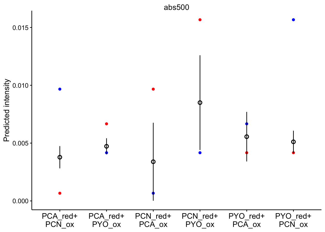
em 460
ggplot(bg_sub_redox %>% filter(wavelength == "em460"), aes(x = red_ox)) +
    geom_point(aes(y = pred_init), color = "red") + geom_point(aes(y = pred_final),
    color = "blue") + geom_pointrange(aes(y = bg_sub, ymin = bg_sub -
    2 * std_per_cond, ymax = bg_sub + 2 * std_per_cond), shape = 21) +
    facet_wrap(~wavelength, scales = "free") + scale_x_discrete(labels = red_ox_labs,
    name = NULL) + theme(axis.text.x = element_text(size = 12)) +
    labs(y = "Predicted intensity")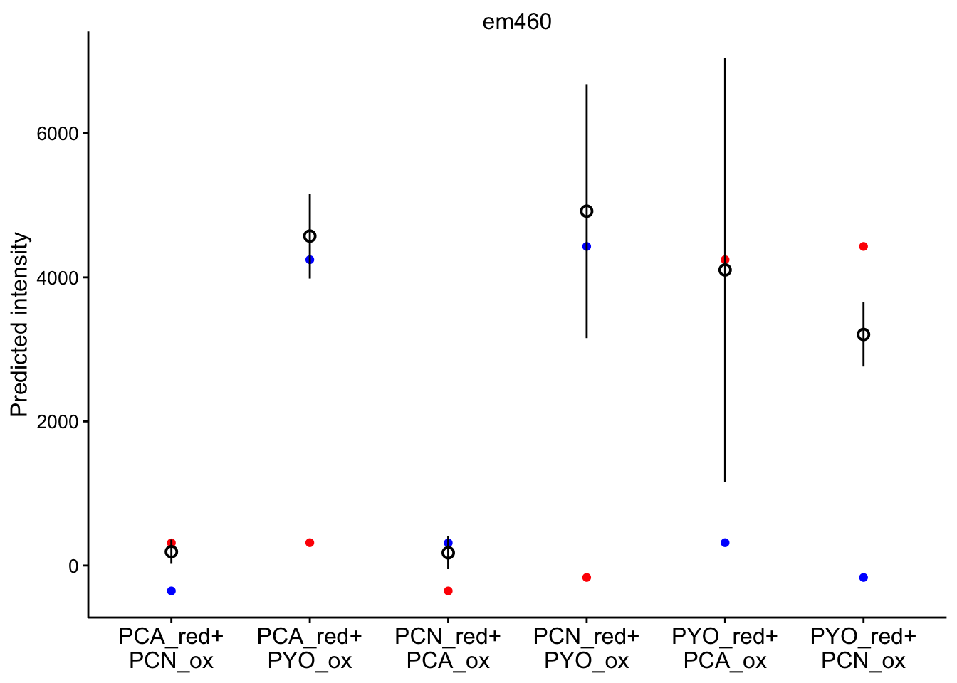
em 528
ggplot(bg_sub_redox %>% filter(wavelength == "em528"), aes(x = red_ox)) +
    geom_point(aes(y = pred_init), color = "red") + geom_point(aes(y = pred_final),
    color = "blue") + geom_pointrange(aes(y = bg_sub, ymin = bg_sub -
    2 * std_per_cond, ymax = bg_sub + 2 * std_per_cond), shape = 21) +
    facet_wrap(~wavelength, scales = "free") + scale_x_discrete(labels = red_ox_labs,
    name = NULL) + theme(axis.text.x = element_text(size = 12)) +
    labs(y = "Predicted intensity")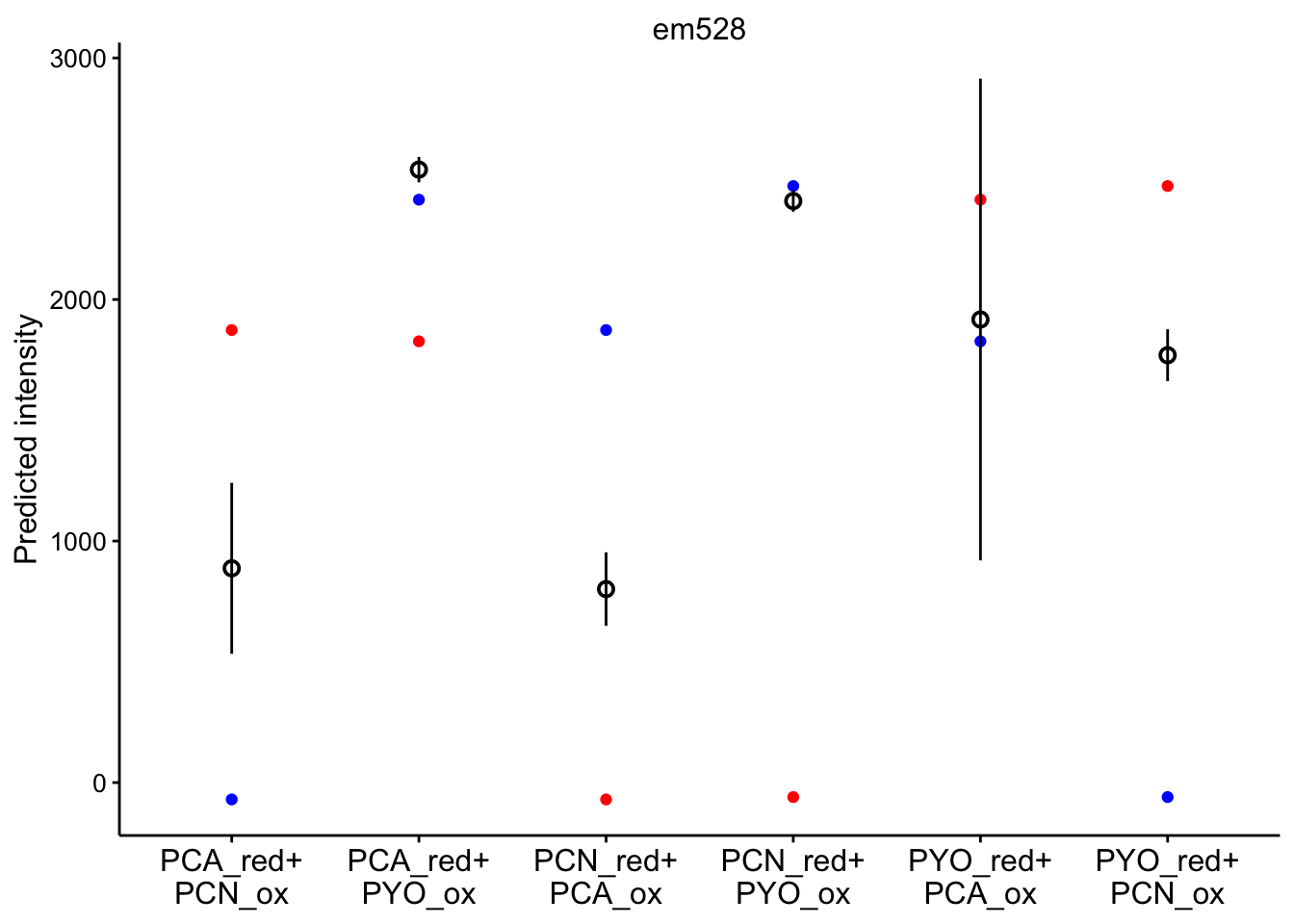
Normalizing for reaction completion
Now let’s normalize!
df_rxn_pct <- bg_sub_redox %>% mutate(rxn_range = abs(pred_final -
    pred_init), rxn_ext = abs(bg_sub - pred_init)) %>% mutate(rxn_ext_high = abs((bg_sub +
    2 * std_per_cond) - pred_init), rxn_ext_low = abs((bg_sub -
    2 * std_per_cond) - pred_init)) %>% mutate(rxn_pct = rxn_ext/rxn_range,
    rxn_pct_high = rxn_ext_high/rxn_range, rxn_pct_low = rxn_ext_low/rxn_range)
Here’s what all the data look like together.
ggplot(df_rxn_pct, aes(x = red_ox, y = rxn_pct, color = wavelength)) +
    geom_pointrange(aes(ymin = rxn_pct_low, ymax = rxn_pct_high),
        position = position_jitter(height = 0, width = 0.1)) +
    scale_x_discrete(labels = red_ox_labs, name = NULL) + scale_y_continuous(labels = scales::percent) +
    labs(y = "Reaction progress")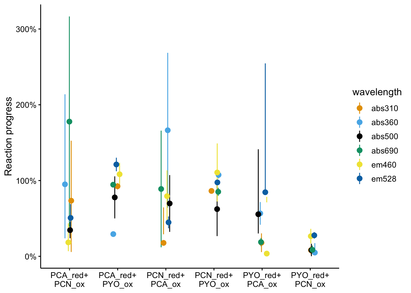
It’s a little hard to parse, especially because certain wavelengths were better for measuring certain phenazines. Here’s the individual wavelengths:
abs310
ggplot(df_rxn_pct %>% filter(wavelength == "abs310"), aes(x = red_ox,
    y = rxn_pct)) + geom_pointrange(aes(ymin = rxn_pct_low, ymax = rxn_pct_high),
    position = position_jitter(height = 0, width = 0.1)) + scale_x_discrete(labels = red_ox_labs,
    name = NULL) + scale_y_continuous(labels = scales::percent) +
    facet_wrap(~wavelength, scales = "free") + labs(y = "Reaction progress")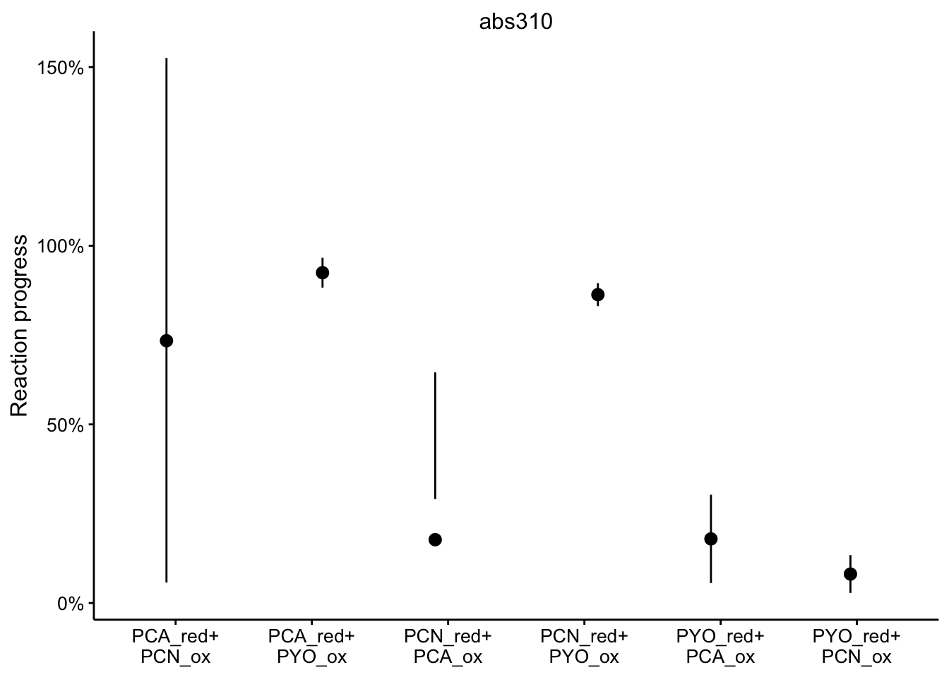
abs360
ggplot(df_rxn_pct %>% filter(wavelength == "abs360"), aes(x = red_ox,
    y = rxn_pct)) + geom_pointrange(aes(ymin = rxn_pct_low, ymax = rxn_pct_high),
    position = position_jitter(height = 0, width = 0.1)) + scale_x_discrete(labels = red_ox_labs,
    name = NULL) + scale_y_continuous(labels = scales::percent) +
    facet_wrap(~wavelength, scales = "free") + labs(y = "Reaction progress")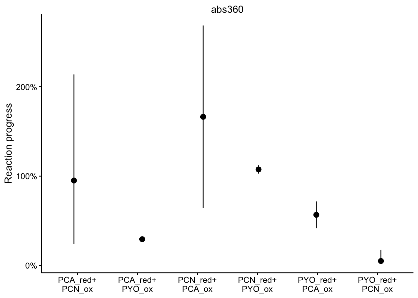
abs690
ggplot(df_rxn_pct %>% filter(wavelength == "abs690"), aes(x = red_ox,
    y = rxn_pct)) + geom_pointrange(aes(ymin = rxn_pct_low, ymax = rxn_pct_high),
    position = position_jitter(height = 0, width = 0.1)) + scale_x_discrete(labels = red_ox_labs,
    name = NULL) + scale_y_continuous(labels = scales::percent) +
    facet_wrap(~wavelength, scales = "free") + labs(y = "Reaction progress")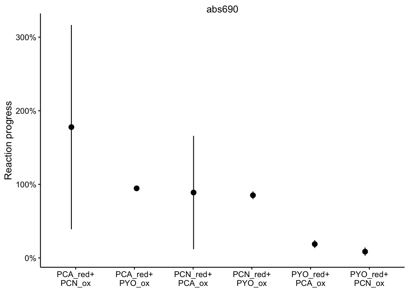
abs500
ggplot(df_rxn_pct %>% filter(wavelength == "abs500"), aes(x = red_ox,
    y = rxn_pct)) + geom_pointrange(aes(ymin = rxn_pct_low, ymax = rxn_pct_high),
    position = position_jitter(height = 0, width = 0.1)) + scale_x_discrete(labels = red_ox_labs,
    name = NULL) + scale_y_continuous(labels = scales::percent) +
    facet_wrap(~wavelength, scales = "free") + labs(y = "Reaction progress")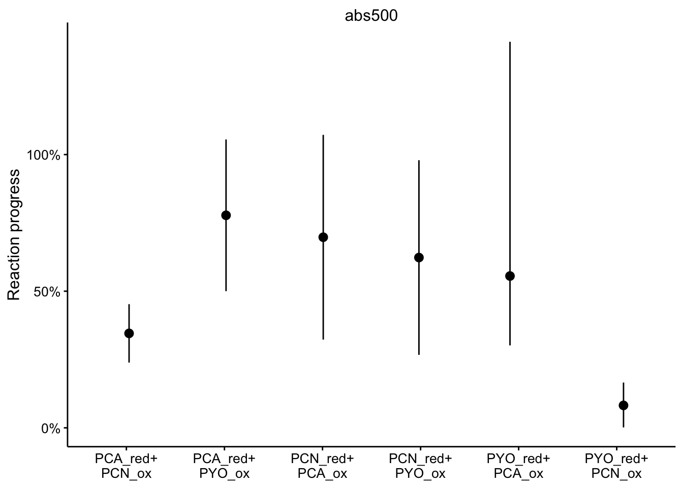
em460
ggplot(df_rxn_pct %>% filter(wavelength == "em460"), aes(x = red_ox,
    y = rxn_pct)) + geom_pointrange(aes(ymin = rxn_pct_low, ymax = rxn_pct_high),
    position = position_jitter(height = 0, width = 0.1)) + scale_x_discrete(labels = red_ox_labs,
    name = NULL) + scale_y_continuous(labels = scales::percent) +
    facet_wrap(~wavelength, scales = "free") + labs(y = "Reaction progress")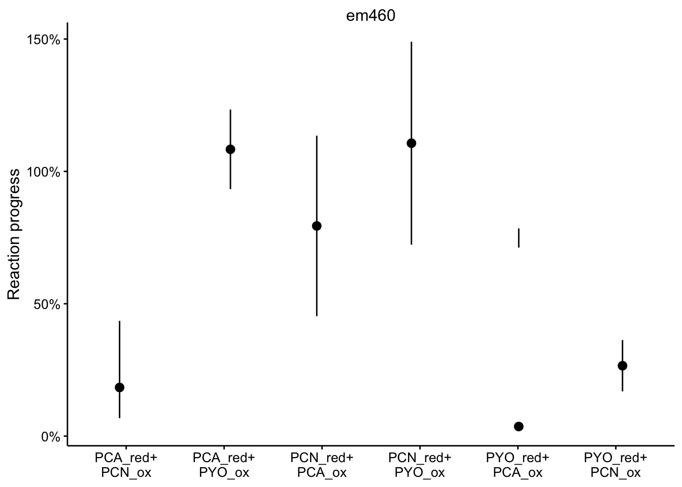
em528
ggplot(df_rxn_pct %>% filter(wavelength == "em528"), aes(x = red_ox,
    y = rxn_pct)) + geom_pointrange(aes(ymin = rxn_pct_low, ymax = rxn_pct_high),
    position = position_jitter(height = 0, width = 0.1)) + scale_x_discrete(labels = red_ox_labs,
    name = NULL) + scale_y_continuous(labels = scales::percent) +
    facet_wrap(~wavelength, scales = "free") + labs(y = "Reaction progress")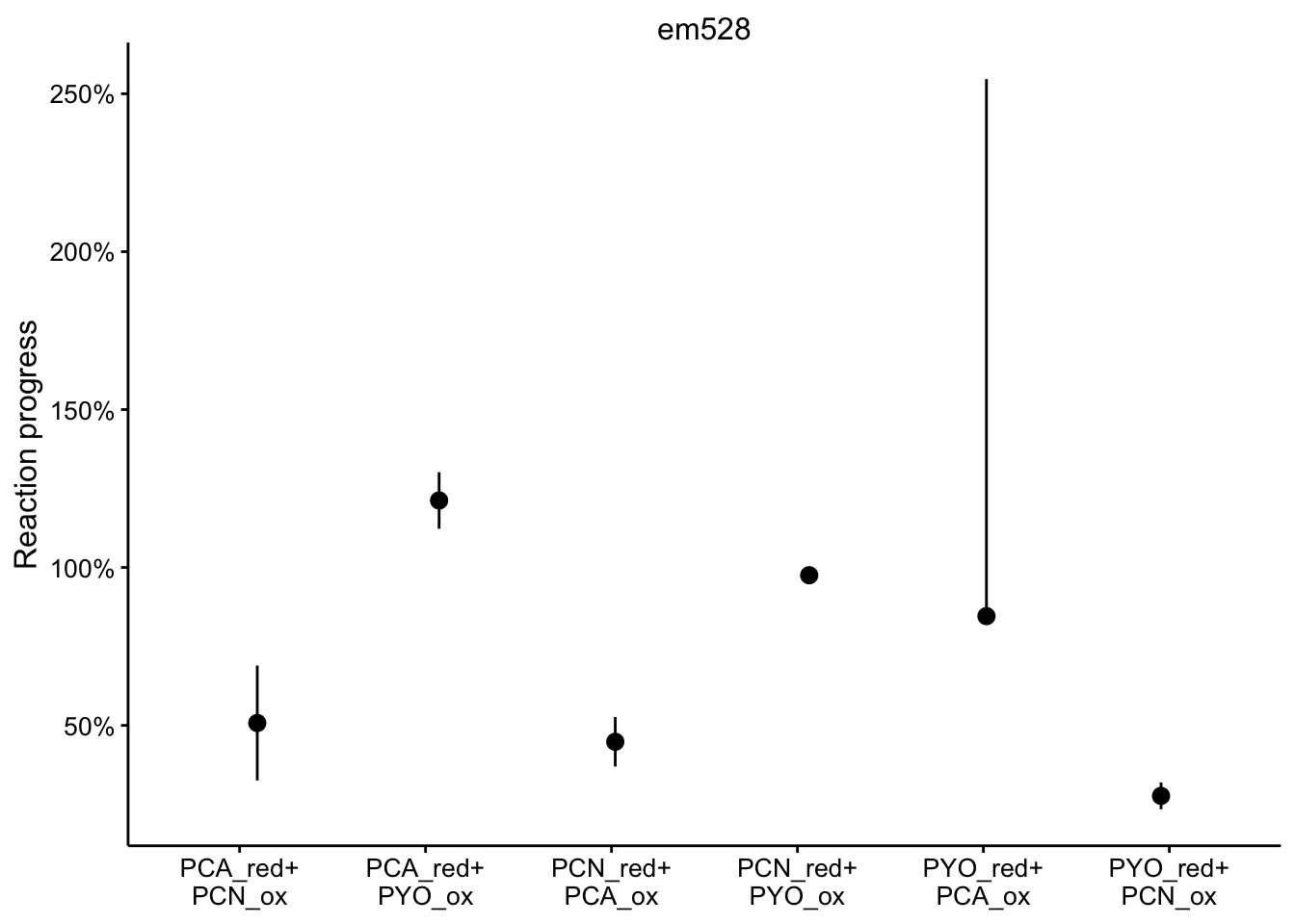
ggplot(df_rxn_pct %>% filter(ox == "PYO") %>% filter(!(wavelength %in%
    c("abs360", "abs500"))), aes(x = red_ox, y = rxn_pct, color = wavelength)) +
    geom_pointrange(aes(ymin = rxn_pct_low, ymax = rxn_pct_high),
        position = position_jitter(height = 0, width = 0.1)) +
    ylim(0, NA)

ggplot(df_rxn_pct %>% filter(red == "PYO") %>% filter(!(wavelength %in%
    c("abs360", "abs500"))), aes(x = red_ox, y = rxn_pct, color = wavelength)) +
    geom_pointrange(aes(ymin = rxn_pct_low, ymax = rxn_pct_high),
        position = position_jitter(height = 0, width = 0.1)) +
    ylim(0, NA)

ggplot(df_rxn_pct %>% filter(red_ox == "PCN_PCA") %>% filter(!(wavelength %in%
    c("abs360", "abs310", "abs690", "abs500"))), aes(x = red_ox,
    y = rxn_pct, color = wavelength)) + geom_pointrange(aes(ymin = rxn_pct_low,
    ymax = rxn_pct_high), position = position_jitter(height = 0,
    width = 0.1)) + ylim(0, NA)

ggplot(df_rxn_pct %>% filter(red_ox == "PCA_PCN") %>% filter(!(wavelength %in%
    c("abs310", "abs690", "abs360"))), aes(x = red_ox, y = rxn_pct,
    color = wavelength)) + geom_pointrange(aes(ymin = rxn_pct_low,
    ymax = rxn_pct_high), position = position_jitter(height = 0,
    width = 0.1)) + ylim(0, 1)

ggplot(df_rxn_pct %>% filter(red_ox == "PYO_PCN") %>% filter(!(wavelength %in%
    c("abs500"))), aes(x = red_ox, y = rxn_pct, color = wavelength)) +
    geom_pointrange(aes(ymin = rxn_pct_low, ymax = rxn_pct_high),
        position = position_jitter(height = 0, width = 0.1)) +
    ylim(0, 1)
Figure draft
It’s hard to concisely represent all of the data, because no single wavelength quantifies all the reactions well. I think the best thing to do is show the 690nm channel tracking the wells that had PYO:
labels = c("PCA[red] + PYO[ox]", "PCN[red] + PYO[ox]", "PYO[red] + PCA[ox]",
"PYO[red] + PCN[ox]")
plot_rxn_pct <- ggplot(df_rxn_pct %>% filter(ox == "PYO" | red ==
"PYO") %>% filter(wavelength == "abs690"), aes(x = red_ox,
y = rxn_pct)) + geom_pointrange(aes(ymin = rxn_pct_low, ymax = rxn_pct_high),
position = position_jitter(height = 0, width = 0.1)) + scale_y_continuous(labels = scales::percent,
limits = c(0, 1)) + labs(y = "Reaction progress at 690nm",
x = NULL) + scale_x_discrete(labels = parse(text = labels)) +
theme(axis.text = element_text(size = 12))
plot_rxn_pct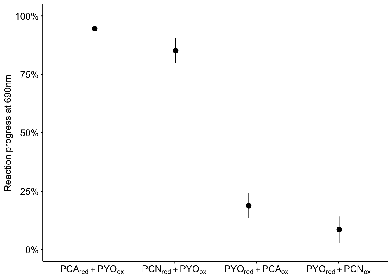 We could potentially add predictions for how far each reaction should go from nernst equation…
As more of a supplemental figure we could show some of the spectra like the spectra comparisons above. (black solid line is PYO_ox and dashed is PYO_red).
plot_pyo_ox <- ggplot(df_ref_4 %>% filter(rep == 1) %>% filter(ox ==
    "PYO"), aes(x = Wavelength, color = red_ox, group = red_ox)) +
    geom_vline(xintercept = 690, color = "gray", linetype = 2) +
    geom_path(aes(y = intensity_phz2_ox), color = "black", linetype = 1) +
    geom_path(aes(y = intensity_phz2_red), color = "black", linetype = 2) +
    geom_path(aes(y = intensity), size = 1) + geom_segment(aes(x = 680,
    xend = 680, y = 0.2, yend = 0.075), arrow = arrow(length = unit(0.05,
    "inches"), type = "closed"), color = "black") + scale_color_manual(labels = parse(text = c("PCA[red] + PYO[ox]",
    "PCN[red] + PYO[ox]")), values = colorblind_palette, name = NULL) +
    labs(y = "Absorbance") + theme(legend.position = "top")


plot_pyo_red <- ggplot(df_ref_4 %>% filter(rep == 1) %>% filter(red ==
    "PYO"), aes(x = Wavelength, color = red_ox, group = red_ox)) +
    geom_vline(xintercept = 690, color = "gray", linetype = 2) +
    geom_path(aes(y = intensity_phz1_ox), color = "black", linetype = 1) +
    geom_path(aes(y = intensity_phz1_red), color = "black", linetype = 2) +
    geom_path(aes(y = intensity), size = 1) + geom_segment(aes(x = 680,
    xend = 680, y = 0.2, yend = 0.075), arrow = arrow(length = unit(0.05,
    "inches"), type = "closed", ends = "first"), color = "black") +
    scale_color_manual(labels = parse(text = c("PYO[red] + PCA[ox]",
        "PYO[red] + PCN[ox]")), values = colorblind_palette,
        name = NULL) + labs(y = "Absorbance") + theme(legend.position = "top")

plot_grid(plot_pyo_ox, plot_pyo_red, align = "hv", axis = "tlbr")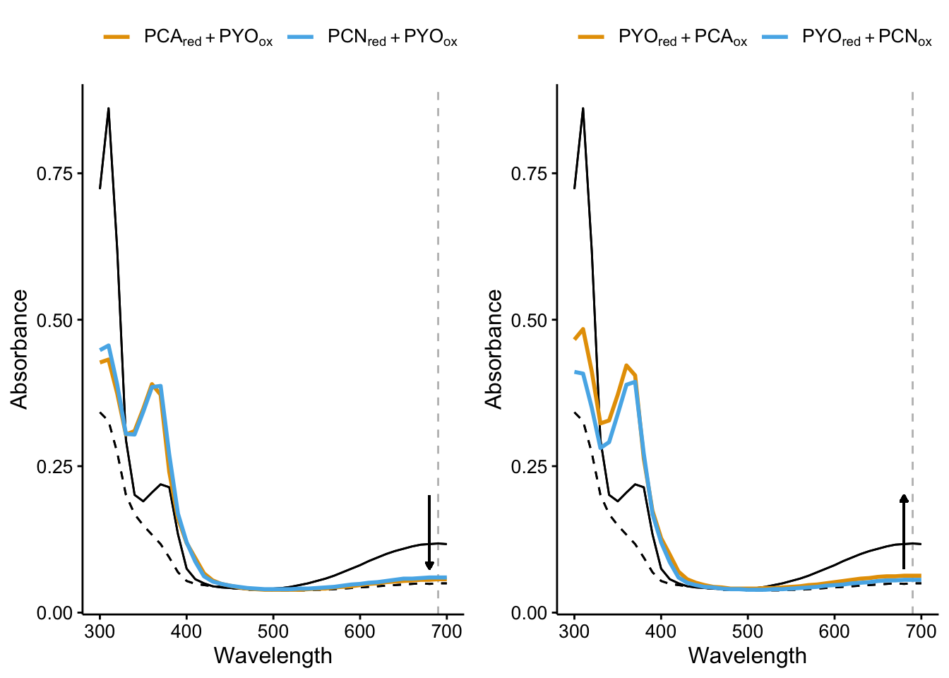
And here’s spectra of all the oxidized and reduced phenazines
plot_phz_ox <- ggplot(df_spectra_meta %>% filter(rep == 1) %>%
    filter(exp == "ref" & red_ox != "PBS_PBS" & phz_redox ==
        "phz_ox"), aes(x = Wavelength, color = phz, group = red_ox)) +
    geom_path(data = df_spectra_meta %>% filter(rep == 1 & red_ox ==
        "PBS_PBS"), aes(x = Wavelength, y = intensity), color = "gray") +
    geom_path(aes(y = intensity), size = 1) + labs(color = NULL) +
    labs(y = "Absorbance", title = "Oxidized phenazines") + theme(legend.position = "top")

plot_phz_red <- ggplot(df_spectra_meta %>% filter(rep == 1) %>%
    filter(exp == "ref" & red_ox != "PBS_PBS" & phz_redox ==
        "phz_red"), aes(x = Wavelength, color = phz, group = red_ox)) +
    geom_path(data = df_spectra_meta %>% filter(rep == 1 & red_ox ==
        "PBS_PBS"), aes(x = Wavelength, y = intensity), color = "gray") +
    geom_path(aes(y = intensity), size = 1) + labs(color = NULL) +
    labs(y = "Absorbance", title = "Reduced phenazines") + theme(legend.position = "top")

plot_grid(plot_phz_ox, plot_phz_red, align = "hv", axis = "tlbr")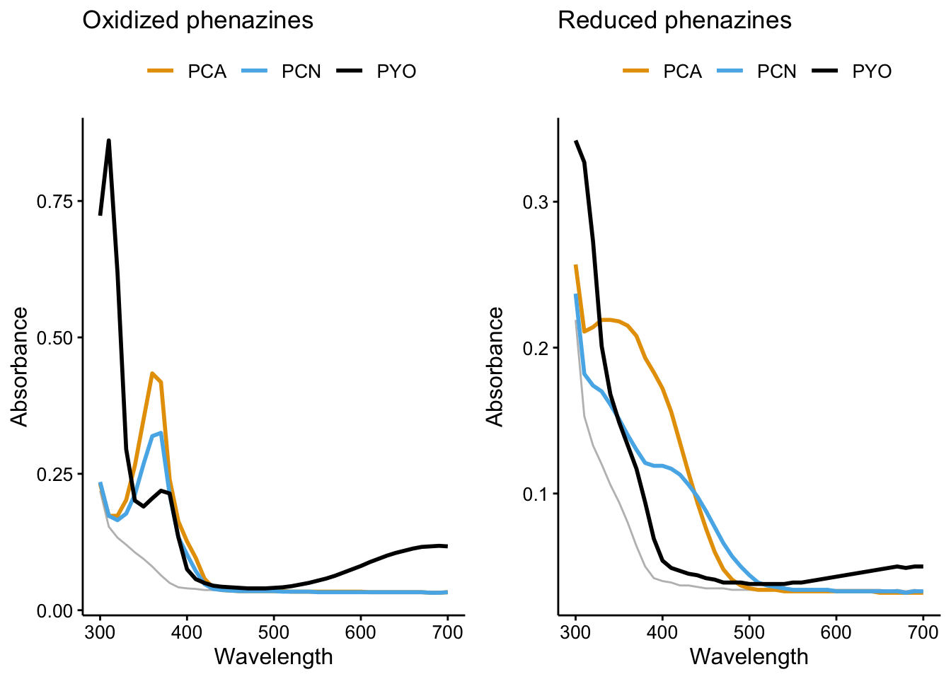
And here’s a nice plot of the predictions at 690nm:
ggplot(bg_sub_redox %>% filter(wavelength == "abs690"), aes(x = red_ox)) +
    geom_point(aes(y = pred_init), color = "red") + geom_point(aes(y = pred_final),
    color = "blue") + geom_pointrange(aes(y = bg_sub, ymin = bg_sub -
    2 * std_per_cond, ymax = bg_sub + 2 * std_per_cond), shape = 21) +
    facet_wrap(~wavelength, scales = "free") + scale_x_discrete(labels = red_ox_labs,
    name = NULL) + theme(axis.text.x = element_text(size = 12)) +
    labs(y = "Predicted intensity")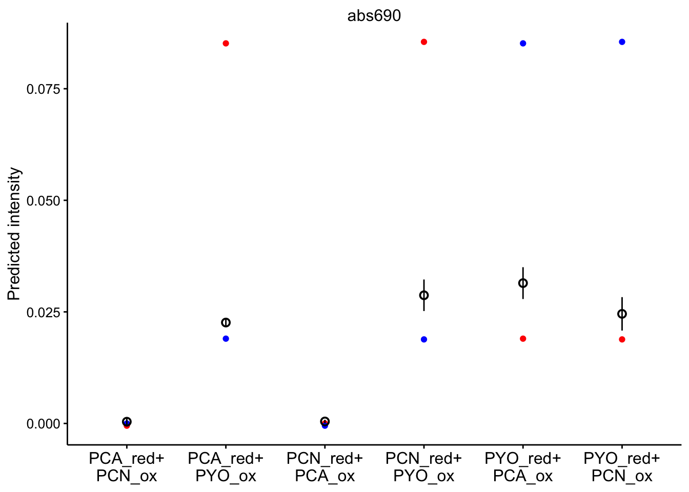
Conclusions
- PYO is rapidly reduced by PCA and PCN in solution
- PCN can kinda reduce PCA and vice versa
- PYO can reduce PCN and PCA a little…as expected from thermodynamics
sessionInfo()## R version 3.5.3 (2019-03-11)
## Platform: x86_64-apple-darwin15.6.0 (64-bit)
## Running under: macOS Mojave 10.14.6
##
## Matrix products: default
## BLAS: /Library/Frameworks/R.framework/Versions/3.5/Resources/lib/libRblas.0.dylib
## LAPACK: /Library/Frameworks/R.framework/Versions/3.5/Resources/lib/libRlapack.dylib
##
## locale:
## [1] en_US.UTF-8/en_US.UTF-8/en_US.UTF-8/C/en_US.UTF-8/en_US.UTF-8
##
## attached base packages:
## [1] stats graphics grDevices utils datasets methods base
##
## other attached packages:
## [1] kableExtra_1.1.0 knitr_1.23 viridis_0.5.1
## [4] viridisLite_0.3.0 cowplot_0.9.4 forcats_0.4.0
## [7] stringr_1.4.0 dplyr_0.8.1 purrr_0.3.2
## [10] readr_1.3.1 tidyr_0.8.3 tibble_2.1.3
## [13] ggplot2_3.2.0 tidyverse_1.2.1
##
## loaded via a namespace (and not attached):
## [1] tidyselect_0.2.5 xfun_0.7 reshape2_1.4.3 haven_2.1.0
## [5] lattice_0.20-38 colorspace_1.4-1 generics_0.0.2 htmltools_0.3.6
## [9] yaml_2.2.0 rlang_0.3.4 pillar_1.4.1 glue_1.3.1
## [13] withr_2.1.2 modelr_0.1.4 readxl_1.3.1 plyr_1.8.4
## [17] munsell_0.5.0 gtable_0.3.0 cellranger_1.1.0 rvest_0.3.4
## [21] evaluate_0.14 labeling_0.3 highr_0.8 broom_0.5.2
## [25] Rcpp_1.0.1 scales_1.0.0 backports_1.1.4 formatR_1.7
## [29] webshot_0.5.1 jsonlite_1.6 gridExtra_2.3 hms_0.4.2
## [33] digest_0.6.19 stringi_1.4.3 grid_3.5.3 cli_1.1.0
## [37] tools_3.5.3 magrittr_1.5 lazyeval_0.2.2 crayon_1.3.4
## [41] pkgconfig_2.0.2 xml2_1.2.0 lubridate_1.7.4 assertthat_0.2.1
## [45] rmarkdown_1.13 httr_1.4.0 rstudioapi_0.10 R6_2.4.0
## [49] nlme_3.1-137 compiler_3.5.3