WT vs ∆PHZ* eDNA, with TOTO
Scott Saunders
11_22_19
library(tidyverse)
library(cowplot)
library(viridis)
library(knitr)
library(kableExtra)
library(modelr)
library(broom)

knitr::opts_chunk$set(tidy.opts=list(width.cutoff=60),tidy=TRUE, echo = TRUE, message=FALSE, warning=FALSE, fig.align="center")

source("../../IDA/tools/plotting_tools.R")

theme_set(theme_1())
Intro
Repeat measurement of eDNA in colonies, but compare WT and ∆phz.
Methods
Six ∆phz* and six WT colony biofilms were grown for four days, as usual. They were resuspended and measured for eDNA using the TOTO plate reader assay as described previously. The dPHZ colonies were a little harder to resuspend, so they received additional vortexing and pipetting.
Basically I acquired 4 plate reader measurements:
- The standard curve with ctDNA
- WT colonies (+ standard curve)
- ∆phz* colonies (+ standard curve)
- Remeasure with ctDNA added to standard wells and first replicate of WT and dPHZ measurements (Wells A1-12, B1-6, E1-6)
The standard curve was made by taking a stock of ctDNA (2mg/mL) and diluting 1:10. That was then used as the highest concentration and was diluted 2x consecutively to fill 12 wells.
The ctDNA added at the end was 2uL of a 1:25 dilution of the 2mg/mL ctDNA stock, because I estimated that should be in the right range to see approximately a doubling of fluorescence.
Results
df_meta <- read_csv("data/2019_11_22_well_metadata.csv")

df_std <- read_csv("data/2019_11_22_std_preCTdna.csv") %>% gather(key = "Well",
    value = "FluorInt", -wavelength) %>% mutate(read = 1)

df_wt <- read_csv("data/2019_11_22_std_WT_preCTdna.csv") %>%
    gather(key = "Well", value = "FluorInt", -wavelength) %>%
    mutate(read = 2)

df_dphz <- read_csv("data/2019_11_22_dphz_preCTdna.csv") %>%
    gather(key = "Well", value = "FluorInt", -wavelength) %>%
    mutate(read = 3)

df_ctDNA <- read_csv("data/2019_11_22_std_wt_dphz_postCTdna.csv") %>%
    gather(key = "Well", value = "FluorInt", -wavelength) %>%
    mutate(read = 4)

df_all <- bind_rows(df_std, df_wt, df_dphz, df_ctDNA)

df_all_meta <- left_join(df_all, df_meta, by = c(Well = "well"))
Calibration curve
ggplot(df_all_meta %>% filter(strain == "std" & wavelength ==
    535), aes(x = well_std_conc, y = FluorInt, color = factor(read))) +
    geom_point() + geom_smooth(method = "nls", formula = y ~
    max * (x^hill)/((Kd^hill) + (x^hill)), method.args = list(start = c(max = 60000,
    hill = 1, Kd = 5)), se = F)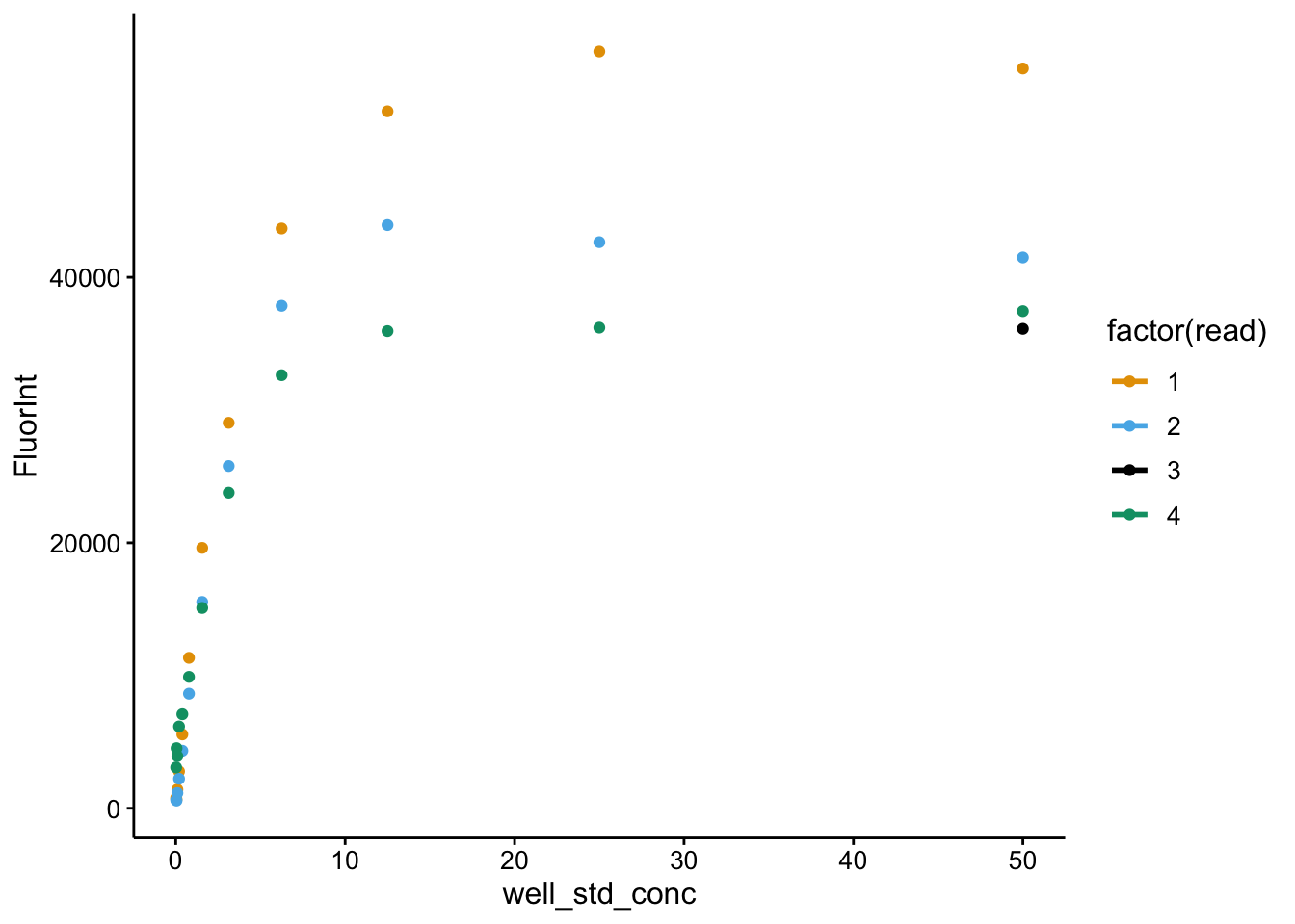
## # A tibble: 12 x 10
##    wavelength Well  FluorInt  read strain toto_added ctDNA_added
##         <dbl> <chr>    <dbl> <dbl> <chr>  <lgl>      <lgl>
##  1        535 A1       55732     1 std    TRUE       TRUE
##  2        535 A2       57010     1 std    TRUE       TRUE
##  3        535 A3       52506     1 std    TRUE       TRUE
##  4        535 A4       43673     1 std    TRUE       TRUE
##  5        535 A5       29038     1 std    TRUE       TRUE
##  6        535 A6       19617     1 std    TRUE       TRUE
##  7        535 A7       11332     1 std    TRUE       TRUE
##  8        535 A8        5564     1 std    TRUE       TRUE
##  9        535 A9        2778     1 std    TRUE       TRUE
## 10        535 A10       1406     1 std    TRUE       TRUE
## 11        535 A11        682     1 std    TRUE       TRUE
## 12        535 A12        774     1 std    TRUE       TRUE
## # … with 3 more variables: well_std_conc <dbl>, bio_rep <dbl>,
## #   tech_rep <dbl>
model_toto <- nls(data = df_all_meta %>% filter(strain == "std" &
wavelength == 535 & read == 1), formula = FluorInt ~ max *
(well_std_conc^hill)/((Kd^hill) + (well_std_conc^hill)),
start = c(max = 60000, hill = 1, Kd = 5))
tidy(model_toto, conf.int = T)## # A tibble: 3 x 7
## term estimate std.error statistic p.value conf.low conf.high
## <chr> <dbl> <dbl> <dbl> <dbl> <dbl> <dbl>
## 1 max 59842. 1473. 40.6 1.65e-11 56876. 63348.
## 2 hill 1.19 0.0780 15.3 9.49e- 8 1.03 1.38
## 3 Kd 2.87 0.211 13.6 2.60e- 7 2.47 3.40confint_toto <- tidy(model_toto, conf.int = T) %>% filter(term ==
"Kd")
pred_toto <- df_all_meta %>% filter(strain == "std" & wavelength ==
535 & read == 1) %>% mutate(max = coef(model_toto)[1], hill = coef(model_toto)[2],
kd = coef(model_toto)[3]) %>% mutate(kd_low = confint_toto$conf.low,
kd_high = confint_toto$conf.high) %>% mutate(pred = max *
(well_std_conc^hill)/((kd^hill) + (well_std_conc^hill))) %>%
mutate(pred_low = max * (well_std_conc^hill)/((kd_low^hill) +
(well_std_conc^hill))) %>% mutate(pred_high = max * (well_std_conc^hill)/((kd_high^hill) +
(well_std_conc^hill)))
ggplot(pred_toto, aes(x = well_std_conc, y = FluorInt)) + geom_ribbon(aes(ymin = pred_low,
ymax = pred_high), fill = "light gray") + geom_line(aes(y = pred),
linetype = 2) + geom_point(shape = 21)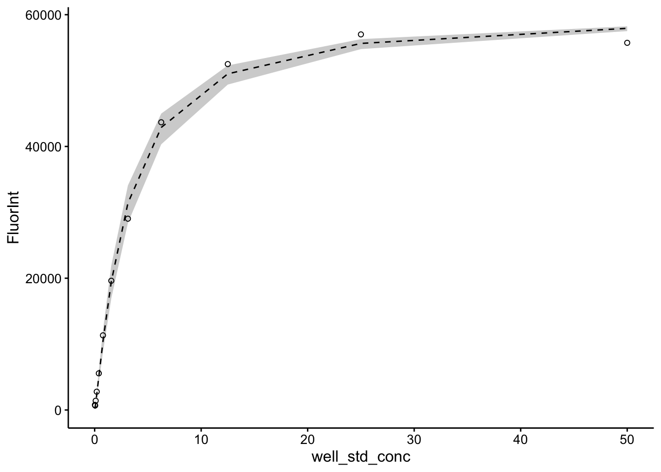
ggplot(pred_toto, aes(x = well_std_conc, y = FluorInt)) + geom_ribbon(aes(ymin = pred_low,
    ymax = pred_high), fill = "light gray") + geom_line(aes(y = pred),
    linetype = 2) + geom_point(shape = 21) + scale_x_log10()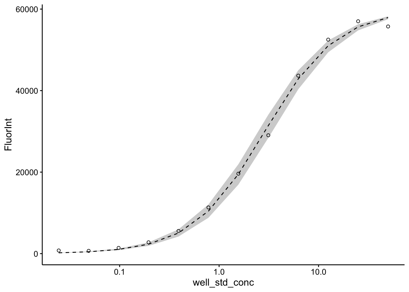
ggplot(pred_toto %>% filter(FluorInt < 30000), aes(x = well_std_conc,
    y = FluorInt)) + geom_ribbon(aes(ymin = pred_low, ymax = pred_high),
    fill = "light gray") + geom_line(aes(y = pred), linetype = 2) +
    geom_point(shape = 21)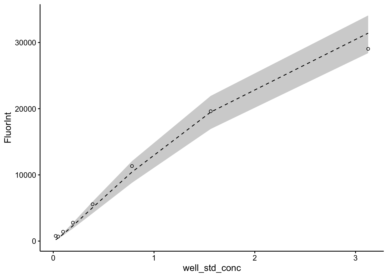
∆phz*
ggplot(df_all_meta %>% filter(strain == "dPHZ" & wavelength ==
    535), aes(x = bio_rep, y = FluorInt, color = factor(read),
    shape = ctDNA_added)) + geom_point() + facet_wrap(~tech_rep)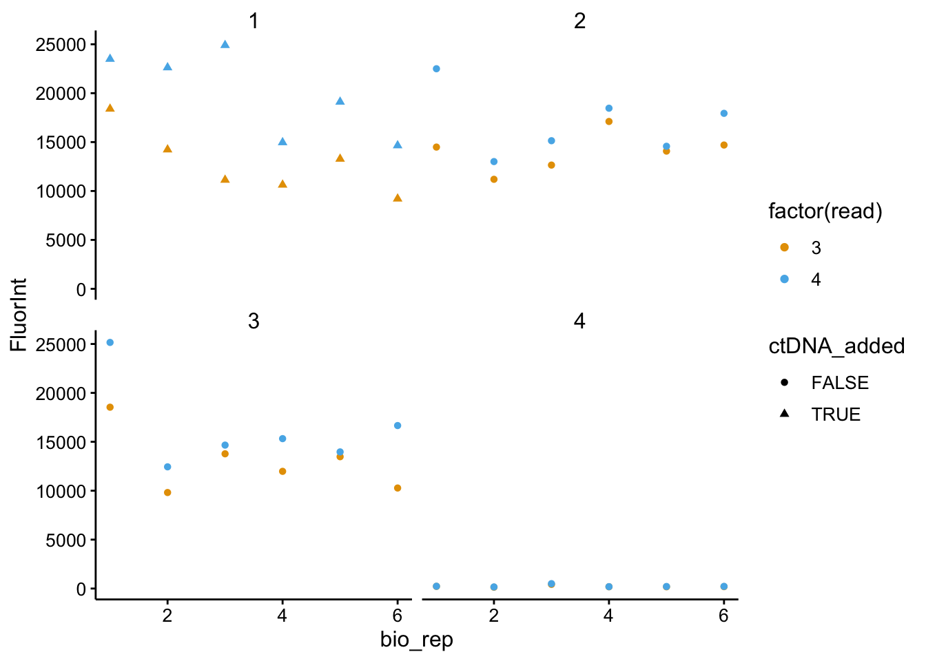
WT
ggplot(df_all_meta %>% filter(strain == "WT" & wavelength ==
    535), aes(x = bio_rep, y = FluorInt, color = factor(read),
    shape = ctDNA_added)) + geom_point() + facet_wrap(~tech_rep)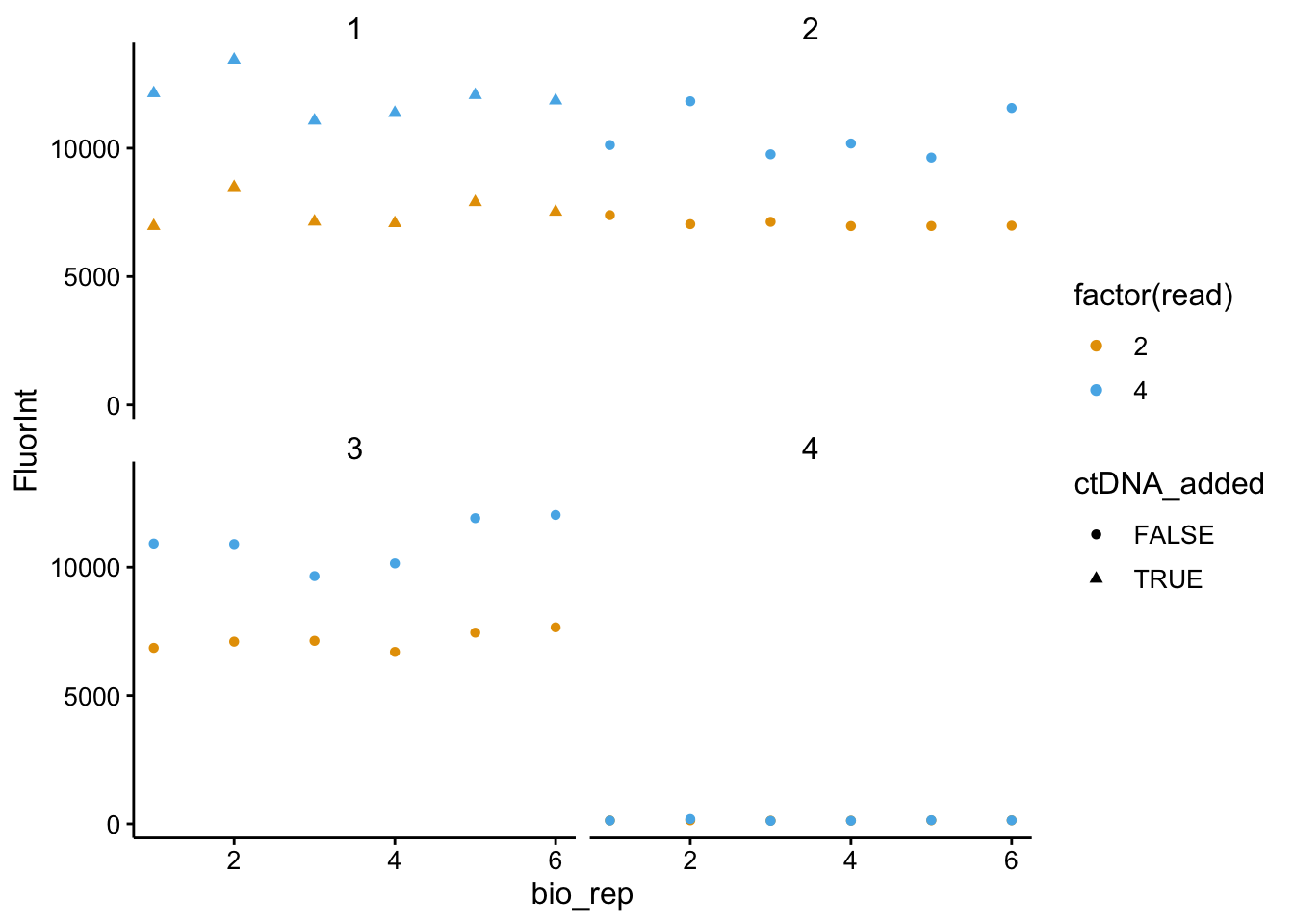
Comparison
df_ctDNA_change <- df_all_meta %>% filter(wavelength == 535) %>%
    group_by(strain, tech_rep, bio_rep, ctDNA_added) %>% summarise(min = min(FluorInt),
    max = max(FluorInt)) %>% mutate(range = max - min)

ggplot(df_ctDNA_change %>% filter(strain != "std" & tech_rep <
    4), aes(x = factor(tech_rep), y = range, shape = ctDNA_added)) +
    geom_point() + facet_wrap(~strain) + scale_shape_manual(values = c(21,
    22))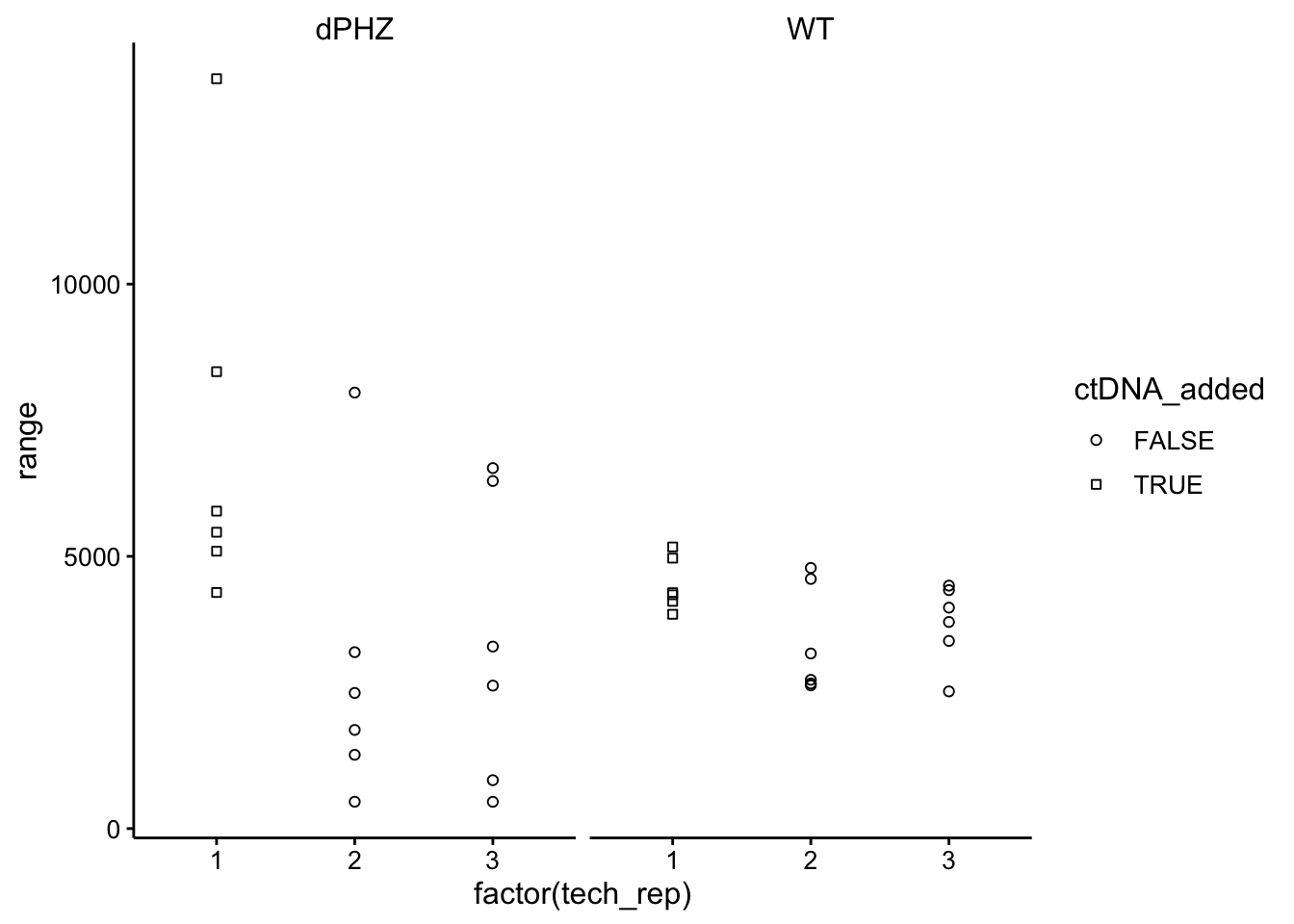
Interestingly, the initial reading for WT was taken more quickly following incubation with the dye than ∆phz, because I had to restart the ∆phz scan because it was taking too long to re-read the WT samples. Perhaps that is the reason all the WT samples increased greatly between the first and last reads.
I think the safest thing to do (in order to compare WT and ∆phz) would be to take the final reading and ignore the technical replicate that had DNA added.
That still gives us 6 biological replicates and 2 tech. reps to work with.
ggplot(df_all_meta %>% filter(strain %in% c("WT", "dPHZ") & wavelength ==
    535 & read == 4 & ctDNA_added == FALSE & toto_added == T),
    aes(x = strain, y = FluorInt)) + geom_boxplot() + geom_jitter(shape = 21,
    height = 0, width = 0.1) + ylim(0, NA)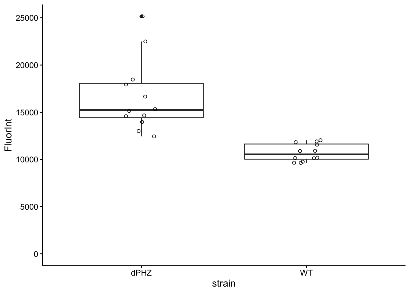
However, adding ctDNA to WT samples did not increase the signal, whereas for ∆phz* samples it did. This suggests that there may be a further complication where the WT biofilms either inhibit the binding of the dye, or degrade the free ctDNA…
## R version 3.5.2 (2018-12-20)
## Platform: x86_64-apple-darwin15.6.0 (64-bit)
## Running under: macOS Mojave 10.14.6
##
## Matrix products: default
## BLAS: /Library/Frameworks/R.framework/Versions/3.5/Resources/lib/libRblas.0.dylib
## LAPACK: /Library/Frameworks/R.framework/Versions/3.5/Resources/lib/libRlapack.dylib
##
## locale:
## [1] en_US.UTF-8/en_US.UTF-8/en_US.UTF-8/C/en_US.UTF-8/en_US.UTF-8
##
## attached base packages:
## [1] stats     graphics  grDevices utils     datasets  methods   base
##
## other attached packages:
##  [1] broom_0.5.1       modelr_0.1.2      kableExtra_1.0.1
##  [4] knitr_1.23        viridis_0.5.1     viridisLite_0.3.0
##  [7] cowplot_0.9.4     forcats_0.3.0     stringr_1.3.1
## [10] dplyr_0.8.1       purrr_0.2.5       readr_1.3.1
## [13] tidyr_0.8.2       tibble_2.1.3      ggplot2_3.2.0
## [16] tidyverse_1.2.1
##
## loaded via a namespace (and not attached):
##  [1] tidyselect_0.2.5 xfun_0.7         haven_2.0.0      lattice_0.20-38
##  [5] colorspace_1.4-0 generics_0.0.2   htmltools_0.3.6  yaml_2.2.0
##  [9] utf8_1.1.4       rlang_0.4.0      pillar_1.3.1     glue_1.3.1
## [13] withr_2.1.2      readxl_1.2.0     munsell_0.5.0    gtable_0.2.0
## [17] cellranger_1.1.0 rvest_0.3.2      evaluate_0.14    labeling_0.3
## [21] fansi_0.4.0      Rcpp_1.0.1       scales_1.0.0     backports_1.1.3
## [25] formatR_1.5      webshot_0.5.1    jsonlite_1.6     gridExtra_2.3
## [29] hms_0.4.2        digest_0.6.18    stringi_1.2.4    grid_3.5.2
## [33] cli_1.1.0        tools_3.5.2      magrittr_1.5     lazyeval_0.2.1
## [37] crayon_1.3.4     pkgconfig_2.0.2  MASS_7.3-51.1    xml2_1.2.0
## [41] lubridate_1.7.4  assertthat_0.2.1 rmarkdown_1.13   httr_1.4.0
## [45] rstudioapi_0.9.0 R6_2.4.0         nlme_3.1-140     compiler_3.5.2